ABSTRACT (original article): Time delays increase the effective dimensionality of reservoirs, thus suggesting that time delays in reservoirs can enhance their performance, particularly their memory and prediction abilities. We find new closed - form expressions for memory and prediction functions of linear time - delayed reservoirs in terms of the power spectrum of the input and the reservoir transfer function. We confirm this relationship numerically for some time - delayed reservoirs using simulations, including when the reservoir can be linearized but is actually nonlinear. Finally, we use these closed - form formulae to address the utility of multiple time delays in linear reservoirs in order to perform memory and prediction, finding similar results to previous work on nonlinear reservoirs. We hope these closed - form formulae can be used to understand memory and predictive capabilities in time - delayed reservoirs. CITATION (original article): Peyton Mullarkey, Sarah Marzen (2025), New analytic formulae for memory and prediction functions in reservoir computers with time delays, arXiv:2503.19806. https://doi.org/10.48550/arXiv.2503.19806
Part 1 of Figure 4
Part 1 of Figure 4
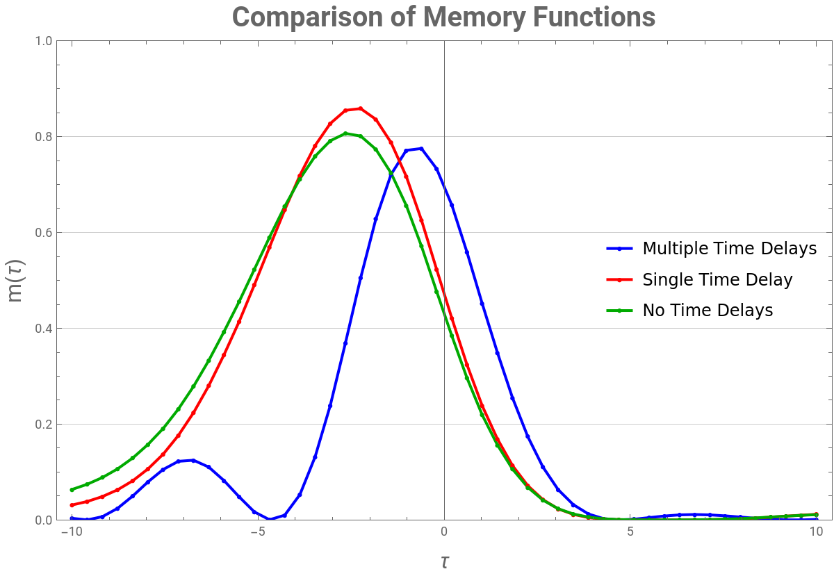
The code below simulates a linear reservoir with chosen delays, measures how well s predicts x across time lags using R², and plots the results to compare the no-delay, single-delay, and multi-delay cases .
- Simulates a noisy, damped oscillator as the input signal.
- Processes it with three linear reservoir setups: no delay, a single delay, and multiple delays.
- Computes a memory function by fitting x shifted in time from s and recording R² across lags.
- Plots the three curves to compare how delays affect memory.
Parameters and grids
In[]:=
alpha=0.2;gamma=0.5;dD=1.;k=0.2;dt=0.01;sdt=Sqrt[dt];T=200.;numSteps=Floor[T/dt];tauValues=Subdivide[-10.,10.,49];
Fixed randomness so runs are reproducible and comparable
In[]:=
SeedRandom[12345];etaMaster=RandomVariate[NormalDistribution[0,1],numSteps-1];(*Simulator:noisySHOdrivingalineardelayedreservoir*)simulateLinearWithEta[delays_List,eta_List]:=Module[{delaySteps=Round[delays/dt],x,v,s,i,d},x=ConstantArray[0.,numSteps];v=ConstantArray[0.,numSteps];s=ConstantArray[0.,numSteps];Do[x[[i]]=x[[i-1]]+v[[i-1]]*dt;(*Euler–Maruyamaupdatesforx,v(noisydampedoscillator)*)v[[i]]=v[[i-1]]+(-alpha*x[[i-1]]-gamma*v[[i-1]])*dt+eta[[i-1]]*dD*sdt;If[delaySteps==={}||delaySteps==={0},(*NOdelaycase*)s[[i]]=s[[i-1]]-k*(s[[i-1]]-x[[i]])*dt,(*MULTI/SINGLEdelaycases*)s[[i]]=s[[i-1]];Do[If[i>d,s[[i]]+=(-k*(s[[i-d]]-x[[i]])*dt),Break[]],{d,delaySteps}]];,{i,2,numSteps}];{x,s}];(*Memorycurve:R^2betweens(t)andtime-shiftedx*)memoryR2FromSeries[x_List,s_List]:=Table[With[{steps=Floor[Abs[tau]/dt]},Module[{delayedX,sShort,lm},(*tau≥0comparess(t)toFUTUREx(t+tau);tau<0comparestoPASTx(t-tau).*)If[tau>=0,delayedX=x[[1+steps;;]];sShort=s[[;;-1-steps]],delayedX=x[[;;-1-steps]];sShort=s[[1+steps;;]]];lm=LinearModelFit[Transpose[{sShort,delayedX}],y,y];lm["RSquared"]]],{tau,tauValues}];
Run with the shared noise so only delays differ
In[]:=
computeMemory[delays_List]:=Module[{x,s},{x,s}=simulateLinearWithEta[delays,etaMaster];memoryR2FromSeries[x,s]];mMulti=computeMemory[{1.,2.,3.}];mSingle=computeMemory[{1.}];mNone=computeMemory[{}];
Plot
In[]:=
ListLinePlot[{Transpose[{tauValues,mMulti}],Transpose[{tauValues,mSingle}],Transpose[{tauValues,mNone}]},Joined->True,PlotMarkers->{{"●",5},{"●",5},{"●",5}},PlotStyle->{Directive[Blue,Thick],Directive[Red,Thick],Directive[Darker[Green],Thick]},Frame->True,GridLines->{{0},Automatic},PlotRange->{0,1},FrameLabel->{Style["τ",16],Style["m(τ)",16]},PlotLegends->Placed[{"Multiple Time Delays","Single Time Delay","No Time Delays"},{Right,Center}],PlotLabel->Style["Comparison of Memory Functions",20,Bold],ImageSize->600]
Out[]=
Below produces a “memory function” 𝑚(𝜏) using the analytic formula for m (τ) in Eq . 13 of the paper for a linear delayed reservoir with multiple time delays driven by a noisy damped oscillator, then plots m(τ) over 𝜏 ∈ [−10,10].
In[]:=
alpha=0.2;k=0.2;d=1;gamma=0.5;newint[tt_]:=ComplexExpand[Re[Exp[-I*ω*tt]*(1*3*(d^2/((ω^2-alpha)^2+ω^2*gamma^2)))/(I*ω+k*(Exp[-I*ω*1]+Exp[-I*ω*2]+Exp[-I*ω*3]))]];numerator[tt_]:=(1/(2*Pi))^2*Re[NIntegrate[Evaluate[newint[tt]],{ω,-∞,∞}]]^2denominator=(1/(2*Pi))*Re@NIntegrate[(1*3)^2*(d^2/((ω^2-alpha)^2+ω^2*gamma^2))/Abs[I*ω+k*(Exp[-I*ω*1]+Exp[-I*ω*2]+Exp[-I*ω*3])]^2,{ω,-∞,∞}]*(1/(2*Pi))*NIntegrate[d^2/((ω^2-alpha)^2+ω^2*gamma^2),{ω,-∞,∞}];data=Table[{T,numerator[T]/denominator},{T,-10,10}];ListPlot[data,Joined->True,PlotRange->{0,1},Frame->True,GridLines->Automatic,FrameLabel->{"τ","m(τ)"}]
Out[]=
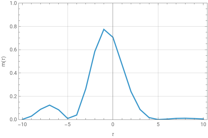
Figure 1
Figure 1
Below I overlay the empirical memory function with the analytic memory function for a linear reservoir with multiple time delays. This code produced Figure 1 in the paper. The plot shows that the analytics match the simulation results.
In[]:=
analyticOnGrid=Transpose@{tauValues,(numerator[#]/denominator)&/@tauValues};empirical=Transpose@{tauValues,mMulti};ListLinePlot[{empirical,analyticOnGrid},Joined->True,PlotMarkers->{{"●",5},None},PlotStyle->{Directive[Blue,Thick],Directive[Red,Thick]},Frame->True,GridLines->{{0},Automatic},PlotRange->{0,1},FrameLabel->{Style["τ",16],Style["m(τ)",16]},PlotLegends->Placed[{"Empirical (R^2)","Analytic"},{Right,Center}],PlotLabel->Style["Comparison of Memory Functions",20,Bold],ImageSize->600]
Out[]=
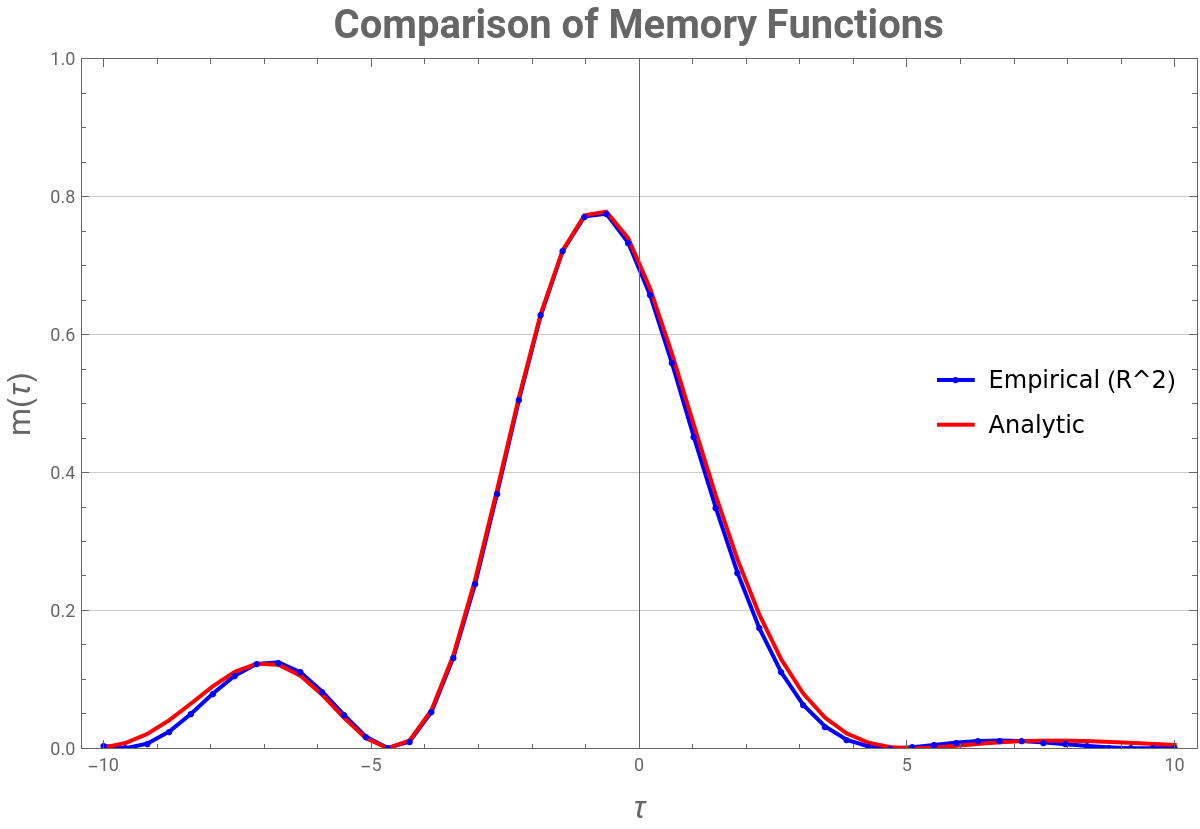
Figure 2
Figure 2
Below calculates uses the analytics to produce the memory function for a linear reservoir with an irrational time delay (π ). This proved that the analytic formula for m (τ) in Eq. 13 of the paper, the memory and prediction function, can handle irrational time delays that would be hard to simulate. Irrational time delays technically lead to an infinite - order reservoir and involve propagating a function rather than a finite number of values. Reservoir and input have parameters k = 0.2, K = 0.2, D = 1, γ = 0.5, and a time delay of π. This produced Figure 2!
ClearAll["Global`*"];alpha=0.2;k=0.2;d=1;gamma=0.5;newint[tt_]:=ComplexExpand[Re[Exp[-I*ω*tt]*(1*3*(d^2/((ω^2-alpha)^2+ω^2*gamma^2)))/(I*ω+k*(Exp[-I*ω*π]))]];numerator[tt_]:=(1/(2*Pi))^2*Re[NIntegrate[Evaluate[newint[tt]],{ω,-∞,∞}]]^2denominator=(1/(2*Pi))*Re@NIntegrate[(1*3)^2*(d^2/((ω^2-alpha)^2+ω^2*gamma^2))/Abs[I*ω+k*(Exp[-I*ω*π])]^2,{ω,-∞,∞}]*(1/(2*Pi))*NIntegrate[d^2/((ω^2-alpha)^2+ω^2*gamma^2),{ω,-∞,∞}];data=Table[{T,numerator[T]/denominator},{T,-10,10}];ListPlot[data,Joined->True,PlotRange->{0,1},Frame->True,GridLines->Automatic,FrameLabel->{"τ","m(τ)"}]
Figure 3
Figure 3
Below is a simulation of a nonlinear reservoir with multiple time delays, as well as code to calculate the approximated memory function for the nonlinear reservoir with multiple time delays. I then overlay my simulated memory function and my approximated memory function to produced Fig . 3. This showed that the analytics match the simulation results even for nonlinear reservoirs that can be linearized.
Simulation
Tau grid and correlation helper
Run with a fixed RNG state
Analytics
Overlay plot
Part 2 of Figure 4
Part 2 of Figure 4
Below is code that shows that difference in memory and prediction for each of these reservoirs can be understood via the difference in transfer functions . All of these transfer functions constitute low - pass filters, but by adding multiple time delays, the low - pass filters acquire oscillatory components, which helps explain why a multiple time delayed reservoir showed to be more advantageous than a single and no time delay reservoir .
CITE THIS NOTEBOOK
CITE THIS NOTEBOOK
New analytic formulae for memory and prediction functions in reservoir computers with time delays
by Peyton Mullarkey & Sarah Marzen
Wolfram Community, STAFF PICKS, September 23, 2025
https://community.wolfram.com/groups/-/m/t/3549742
by Peyton Mullarkey & Sarah Marzen
Wolfram Community, STAFF PICKS, September 23, 2025
https://community.wolfram.com/groups/-/m/t/3549742