In this project, I examined the complexities of 2-color 2-state 2D Turing machines, the simplest possible 2D Turing Machine rules that encompass all four 2D directions. To start, I did background research on existing rules for 2D Turing machines, like Langton's Ant. I sought to systematically consider the complexities of 2-color 2-state rules, so I generated all the 65,536 possible rule, but removed all rules that resulted in one-dimensional movement, to have a list of roughly 20,000 rules. After I generated the rules, I designed three methods to test and quantify the complexities of each rule. The first considered the ratio of the length and width of the final grid after 100 evolutions of the rule, and considered the more "square" ones to be more complex. The second ranked the complexities of the rules based on the standard deviations of the lengths of the largest blocks of the rows in the grids. The third eliminated rules that didn't have enough long blocks, which are simple. The results of the complexity search led me to conjecture that all 2-color 2-state 2D Turing machines with blank initial states are simple, and fall into an infinitely repeating pattern within just a few steps.
Background on Turing Machines
Background on Turing Machines
General Description
General Description
Turing machines, TM for short, are an abstract model of a computation device designed by Alan Turing. They contain two basic components, the head and the tape. The head is a machine with a finite number of possible states that moves along the tape, which is infinitely long and divided into cells, each of which has a finite number of possible states, often called colors. As the head moves along the tape, it compares the state of the head and color of the cell with a table of rules, which dictate how the state and color should change and where the head should move next.
A two-dimensional TM works exactly the same, except instead of moving along a tape of width 1, the head moves on an infinitely large grid.
A two-dimensional TM works exactly the same, except instead of moving along a tape of width 1, the head moves on an infinitely large grid.
Langton's Ant
Langton's Ant
Basic Description
Basic Description
Possibly the most famous two-dimensional TM is Langton's Ant, a 4-state 2-color TMs . The head, also called the ant, has four states, representing the direction the ant is facing. When the ant is on a white square, it turns left, and when it is on a black square, it turns right. After turning, it always moves forward one step to the next cell, and changes the previous cell to the opposite color.
The following defines the rules for Langton's Ant:
In[]:=
directions={{1,0},{0,1},{-1,0},{0,-1}};twoRule=Flatten[Table[{a,b}->{If[b==1,Mod[a,4]+1,Mod[a+2,4]+1],Abs[1-b],If[b==0,directions[[Mod[a,4]+1]],directions[[Mod[a+2,4]+1]]]},{a,1,4},{b,0,1}]]
Out[]=
{{1,0}{4,1,{0,1}},{1,1}{2,0,{0,-1}},{2,0}{1,1,{-1,0}},{2,1}{3,0,{1,0}},{3,0}{2,1,{0,-1}},{3,1}{4,0,{0,1}},{4,0}{3,1,{1,0}},{4,1}{1,0,{-1,0}}}
The Manipulate function can help us better understand how the Langton's Ant behaves, showing the progression of the head and tape step by step.
A Manipulate of Langton's Ant for 1000 steps:
In[]:=
ListAnimate[Table[Show[ArrayPlot[Reverse[Transpose[TuringMachine[twoRule,{1,{{{}},0}},n][[-1,-1]]]]],Graphics[Style[Line[Table[TuringMachine[twoRule,{1,{{{}},0}},n][[i]][[1]][[2]]-{0.5,0.5},{i,n}]],Red]]],{n,1,100,1}]]
Out[]=
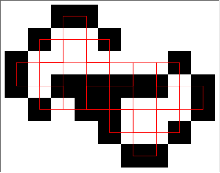
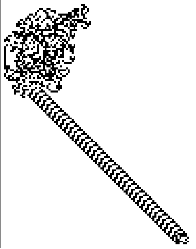
Despite its simple rules, Langton's Ant displays astonishingly complex behavior. For the first ~10,000 steps there is seemingly no order. Then, a pattern suddenly forms, with the ant traveling down a repeating "highway" infinitely.
Langton's Ant after 14,000 steps, with a highway formation on the lower right:
In[]:=
ArrayPlot[Reverse[Transpose[TuringMachine[twoRule,{1,{{{}},0}},14000][[-1,-1]]]]]
Out[]=
A Different Angle
A Different Angle
Despite what looks to be unruly chaos of the Turing Machine tape at the start, looking at the model from a different angle reveals something completely different. Looking at the path of the head instead of the colors on the tape unveils newfound symmetry. In particular, steps such as 100 and 361 are symmetric about the origin. As a side note, the fact that 100 and 361 are both perfect squares seems to be a coincidence, as there are symmetrical paths
Showing only the path of the head after 100 steps:
In[]:=
Graphics[Style[Line[Table[TuringMachine[twoRule,{1,{{{}},0}},100][[i]][[1]][[2]]-{0.5,0.5},{i,100}]],Red]]
Out[]=
Showing only the path of the head after 361 steps :
In[]:=
Graphics[Style[Line[Table[TuringMachine[twoRule,{1,{{{}},0}},361][[i]][[1]][[2]]-{0.5,0.5},{i,361}]],Red]]
Out[]=
Langton's Ant can be classified as a complex, interesting rule, with its almost unpredictable start, and highway formation thousands of steps later. Our goal is to learn more about the complexities of various rules.
2-color 2-state 2D TM Rule Generation
2-color 2-state 2D TM Rule Generation
Some of the simplest 2D Turing Machines are 2-color 2-state. This means each cell is one of two colors, denoted as 0 and 1 (white and black), and the head is always in one of two possible states, also called 0 and 1. Note that this means the cell and head together can be in one of 4 possible states: (0,0), (0,1), (1,0), and (1,1), which can form a one-to-one association with the four possible cardinal directions for head travel. Simple calculations give that there are 2^16=65536 different 2-color 2-state TM rules. This simple calculation includes cases where multiple inputs correspond to the same output. To systematically consider complexity of the rules, the first step is to generate all the possible rules. From here forward, the name of a rule will be its index in the complete list of rules, showAll.
showAll is a generated list of all possible 2-color 2-state rules for a 2D TM:
In[]:=
directions25={{1,0},{0,1},{-1,0},{0,-1}};posStates2={{0,0},{0,1},{1,0},{1,1}};showAll=Flatten[Table[{{0,0}->{p[[1]],p[[2]],a},{0,1}->{q[[1]],q[[2]],b},{1,0}->{r[[1]],r[[2]],c},{1,1}->{s[[1]],s[[2]],d}},{a,directions25},{b,directions25},{c,directions25},{d,directions25},{p,posStates2},{q,posStates2},{r,posStates2},{s,posStates2}],7];
Of these 65,536 possible rules, ~40,000 of them can be immediately eliminated, as the final 2D array of the tape colors after 5 steps only has 1 row, meaning the TM moves along a straight line, and is therefore one-dimensional and doesn't employ movement in all four directions.
noZeros contains the names of all rules that expand to at least 2 rows after 5 steps, with goodRules being a helper list to generate noZeros:
In[]:=
goodRules={};Flatten[Table[If[(Length[TuringMachine[showAll[[i]],{1,{{{}},0}},5][[-1,-1]]]!=1)&&(Length[TuringMachine[showAll[[i]],{1,{{{}},0}},5][[-1,-1]][[1]]]!=1),Append[goodRules,i],0],{i,Range[2^16]}]];noZeros=Select[goodRules2,#!=0&];
Finding and Quantifying Complexity in 2-color 2-state 2D TM Behavior
Finding and Quantifying Complexity in 2-color 2-state 2D TM Behavior
Eliminating Rules Based Off the Proportions of the Final Grid
Eliminating Rules Based Off the Proportions of the Final Grid
To further narrow the list of rules we must run, let us consider the final shape of the grid. Take the case of Langton's Ant, which starts very chaotic and complex. Throughout all the evolutions, the grid remains close to a square; that is, the ratio of the number of rows and the number of columns always stays close to 1.
Upon further consideration, it is reasonable to claim that most complex rules should result in relatively "square" grids after a large enough number of steps, like 100, because in a chaotic and random Turing Machine, the head should move roughly the same amount horizontally and vertically. A simplified calculation of the "squareness" of a rule is just the difference in length and width of the final grid.
Upon further consideration, it is reasonable to claim that most complex rules should result in relatively "square" grids after a large enough number of steps, like 100, because in a chaotic and random Turing Machine, the head should move roughly the same amount horizontally and vertically. A simplified calculation of the "squareness" of a rule is just the difference in length and width of the final grid.
findSquareness returns smaller numbers for more square grids and larger numbers for less square grids, and is mapped across noZeros:
The result is threaded into an association indexSquares with the names of the rule corresponding to the squareness:
It is clear after looking at a few of the the rules with squareness 0 that the grid most often becomes a perfect square when the head just travels in a diagonal line of slope +/-1. So, we rule out all the elements of indexSquares with value 0. Similarly, elements with values 1 and 2 are most likely diagonal lines or steps that required a couple of steps to fall into the pattern.
isGreater2 tests if the input is greater than 2, and only those with True as the output for isGreater2 are selected to join notDiagonals:
The first elements of notDiagonals have value 18 after 100 steps. Running the rule reveals that the squareness 18 rules aren't actually complex. Below is just one of many examples.
Showing the result of the first rule listed in notDiagonals after 100 steps:
So, eliminating rules with too high or low squareness values doesn't clearly reveal any complex 2-color 2-state 2D TMs.
Ranking Complexity Based off Variance in Lengths of Blocks Between Rows
Ranking Complexity Based off Variance in Lengths of Blocks Between Rows
Another way to quantify complexity in a Turing Machine is calculating how much the lengths of black blocks vary between different rows. Specifically, we can find the length of the longest chain of consecutive black squares for each row, and calculate the standard deviation of them, which we will call the complexity value in this section.
Finding all blocks of consecutive black cells and calculating the standard deviation between largest blocks of different rows:
Now that we have found the desired standard deviations for each rule, we can thread an association of the names of the rules and the complexity values, which in this case is the standard deviation. Higher complexity values correspond to more uneven distributions of blocks across rows, which should mean more chaotic and complex behavior. So, we sort the association by the complexity values from largest to smallest, and the rules at the front should be the most complex.
theAcCOmplex threads together the names of rules and complexity values of the rules in an association:
Now, we want to see how a few of the "most complex" rules look according to this method of complexity calculation, to determine how complex they really are.
A few “complex” rules after 20 steps:
The resulting tapes display no complex behavior or chaos, simply coloring in straight lines of width 1 instead. Yet, they are all tied as most complex through this complexity measurement method. So, using the variations in length of blocks in the final grid to test for complexity also gives uninteresting results to be the most complex.
Eliminating Rules Rased Off of Block Lengths in Rows
Eliminating Rules Rased Off of Block Lengths in Rows
The final method used to determine complexity of a rule was to consider the lengths of the first block of consecutive black cells in each of the rows of the final grid. After observing many diagonal lines and stair-like shapes, it became clear that one common type of simple rule resulted in blocks of length less than 3 in every row.
Additionally, another main class of simple rules is rules that result in a strip of black cells that either has width 1 or 2. So, if only tested to see if grids have blocks of length 3, those simple rules would slip through the test and be considered complex. So, we must also consider how many rows have blocks of length 3, and that should be at least 3.
Also, technical limitations prevent us from iterating through all the blocks in the grid, so instead we only look at the first one. But, we only require 3 long blocks, so the test should still be relatively complete despite the simplification.
Using findBlock as defined in the previous section, the function isGold tests a rule to see if it has enough long blocks:
seeAll contains all the elements of noZero that have enough long blocks:
Running the elements of seeAll in TuringMachine reveals that once again, even the supposedly more complex 2-color 2-state 2D TMs are simple.
Resulting Conjecture
Resulting Conjecture
For some unknown integer n, any 2-color 2-state two-dimensional Turing Machine with a blank initial state must enter a repeating pattern by the nth evolution of the machine.
Evidence
Evidence
The previous sections tested for complex rules among the complete set of 2-color 2-state rules in multiple different ways, all to no avail. The three methods were all very different, with one focusing on the shape of the overall grid, one focusing on the variation of block length, and the last focusing on the number of long blocks. None could find a rule that demonstrates complex behavior, which logically leads to the question of if any such rules even exist at all.
Possible Proof Paths
Possible Proof Paths
◼
There are very few possible combinations of states the head and cell can be in. Eventually the states repeat, and if it is on a new cell the overall situation of the system looks like the beginning again.
◼
Maybe not all directions can be used in a single rule if the tape starts out blank, in which case it is much harder for complex behavior to occur.
Future Exploration
Future Exploration
In the future, I'd like to complete a rigorous proof of my conjecture that all 2-color 2-state 2D Turing Machines are simple. I’d also like to try generating complex behavior from some of these simple rules by modifying the initial state of the tape and changing the amount the head moves at each step.
Acknowledgements
Acknowledgements
I'd like to thank my mentor Jeremy and all the wonderful staff at the Wolfram Summer Research Program for their help and support. An additional thanks to Stephen Wolfram for the guidance on this project.
References
References
◼
Blum, M., and C. Hewitt. “Automata on a 2-Dimensional Tape.” 8th Annual Symposium on Switching and Automata Theory (SWAT 1967), 1967, https://doi.org/10.1109/focs.1967.6.
◼
“Langton’s Ant.” From Wolfram MathWorld, mathworld.wolfram.com/LangtonsAnt.html. Accessed 13 July 2023.
◼
Pegg, Ed. “2D Turing Machines.” Math Games: 2d Turing Machines, 7 June 2004, www.mathpuzzle.com/MAA/21-2D%20Turing%20Machines/mathgames_06_07_04.html.
◼
Stanica, George Cosmin, and Petre Anghelescu. “Research and Implementation of a Two-Dimensional Cellular Automaton.” 2022 14th International Conference on Electronics, Computers and Artificial Intelligence (ECAI), 2022, https://doi.org/10.1109/ecai54874.2022.9847412.
◼
Szepietowski, Andrzej. “On Three-Way Two-Dimensional Turing Machines.” Information Sciences, vol. 47, no. 2, 1989, pp. 135–147, https://doi.org/10.1016/0020-0255(89)90010-8.
◼
“Turing Machine 2D.” NetLogo Models Library: Turing Machine 2D, ccl.northwestern.edu/netlogo/models/TuringMachine2D. Accessed 13 July 2023.
◼
“Turing Machine.” From Wolfram MathWorld, mathworld.wolfram.com/TuringMachine.html. Accessed 13 July 2023.
◼
Wolfram, Stephen. A New Kind of Science. Wolfram Media, 2021.
CITE THIS NOTEBOOK
CITE THIS NOTEBOOK
Complex behavior in 2-color 2-state 2D Turing machines
by Joyce Huang
Wolfram Community, STAFF PICKS, July 13, 2023
https://community.wolfram.com/groups/-/m/t/2964778
by Joyce Huang
Wolfram Community, STAFF PICKS, July 13, 2023
https://community.wolfram.com/groups/-/m/t/2964778