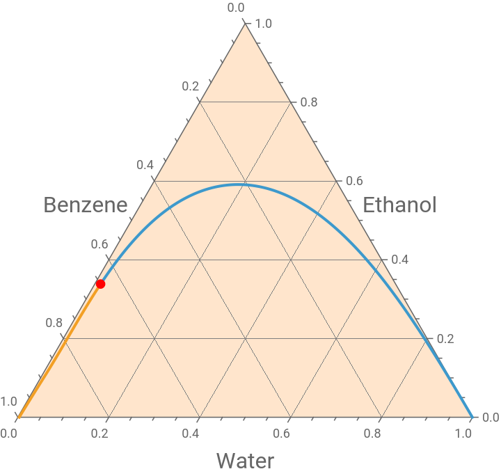
The liquid-liquid equilibrium (LLE) behavior of the ternary water–ethanol–benzene system at 25 °C was investigated using the NRTL activity coefficient model. The common tangent plane (CTP) equations were first solved to obtain an initial tie line, and an arc-length continuation procedure was then applied to trace the entire binodal curve. This approach generated both branches of the coexistence region and allowed the determination of all equilibrium tie lines without repeatedly solving independent equilibrium problems.
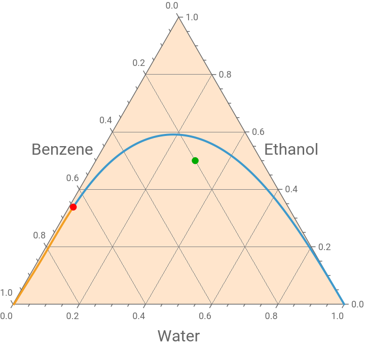
The thermodynamic stability of a feed composition (z={0.30,0.20,0.50}) was then examined using the tangent plane distance (TPD) criterion. The global minimization yielded (TPD_{min}=-0.169529), indicating that the mixture is thermodynamically unstable and will spontaneously split into two liquid phases. The corresponding incipient phase composition was found to be (w*={0.00284,0.96852,0.02864}), confirming that the feed composition lies inside the two-phase region.
The equilibrium tie line passing through this unstable feed was subsequently determined using two independent methods. First, a classical liquid-liquid equilibrium calculation based on equality of component activities and mass balances was solved using FindRoot. Second, the tie line was extracted directly from the arc-length continuation solution. Both approaches produced identical equilibrium compositions, namely (x_alpha={0.33885,0.11096,0.55018}) and (x_beta={0.00753,0.87025,0.12222}), validating the robustness and accuracy of the continuation-based CTP method.
A second feed composition, (z={0.10,0.10,0.80}), was also analyzed to verify the stability criterion outside the miscibility gap. In this case, the TPD minimization yielded (TPD_{min}=2.34*10^-16), which is effectively zero, and the minimizing composition coincided with the feed itself. Therefore, the mixture is thermodynamically stable and remains as a single liquid phase.
These results demonstrate the capability of the combined CTP, arc-length continuation, and TPD framework to distinguish stable and unstable regions and to accurately characterize liquid-liquid phase behavior in ternary systems.
LLE diagram using the method based on common tangent plane and arc-length continuation
In[]:=
ClearAll["Global`*"];
Temperature
TK=273.15+25;
NRTL PARAMETERS -- Source: Aspen-Plus v .14
In[]:=
t13=A13+B13/TK;t23=A23+B23/TK;t12=A12+B12/TK+E12Log[TK];t32=A32+B32/TK;t31=A31+B31/TK;t21=A21+B21/TK+E21Log[TK];
In[]:=
param={a12->0.2,a13->0.30,a32->0.3,B21->591.3676,B12->-5954.3071,A12->140.0874,A21->45.1905,E12->-20.0254,E21->-7.5629,B23->882.0288,B32->-54.8044,A32->0.5686,A23->-0.9155,B13->-586.0809,B31->246.18,A13->3.4578,A31->-0.8009};
NRTL tau_{ij} matrix (dimensionless, at T ≈ 298 K
τ={{0.0,t12,t13},{t21,0.0,t23},{t31,t32,0.0}}/.param;α={{0.0,0.2,0.3},{0.2,0.0,0.3},{0.3,0.3,0.0}};
In[]:=
α//MatrixForm
Out[]//MatrixForm=
0. | 0.2 | 0.3 |
0.2 | 0. | 0.3 |
0.3 | 0.3 | 0. |
In[]:=
τ//MatrixForm
Out[]//MatrixForm=
0. | 6.0199 | 1.49208 |
4.0836 | 0. | 2.04284 |
0.0247918 | 0.384785 | 0. |
G[i_,j_]:=Exp[-α[[i,j]]τ[[i,j]]];
Composition vector
xvec[x1_,x2_]:={x1,x2,1-x1-x2};
NRTL Activity coefficients
lnGamma[i_,x1_,x2_]:=Module[{x,term1,term2},x=xvec[x1,x2];term1=Sum[x[[j]]τ[[j,i]]G[j,i],{j,1,3}]/Sum[x[[k]]G[k,i],{k,1,3}];term2=Sum[x[[j]]G[i,j]/Sum[x[[k]]G[k,j],{k,1,3}](τ[[i,j]]-Sum[x[[m]]τ[[m,j]]G[m,j],{m,1,3}]/Sum[x[[m]]G[m,j],{m,1,3}]),{j,1,3}];term1+term2];gamma[i_,x1_,x2_]:=Exp[lnGamma[i,x1,x2]];
Dimensionless Gibbs energy of mixing: g/RT
gmix[x1_,x2_]:=Module[{x},x=xvec[x1,x2];Sum[x[[i]]Log[x[[i]]],{i,1,3}]+Sum[x[[i]]lnGamma[i,x1,x2],{i,1,3}]];
Derivatives
dgdx1[x1_,x2_]:=Evaluate[D[gmix[u,v],u]/.{u->x1,v->x2}];dgdx2[x1_,x2_]:=Evaluate[D[gmix[u,v],v]/.{u->x1,v->x2}];
Unknowns
vars={x1a,x2a,x1b,x2b,m1,m2};
Common tangent equations
eq1=dgdx1[x1a,x2a]-m1==0;eq2=dgdx1[x1b,x2b]-m1==0;eq3=dgdx2[x1a,x2a]-m2==0;eq4=dgdx2[x1b,x2b]-m2==0;eq5=gmix[x1b,x2b]-gmix[x1a,x2a]==(m1(x1b-x1a)+m2(x2b-x2a));
Extra constraint - Prevent trivial solution xα=xβ
In[]:=
eq6=(x1b-x1a)^2+(x2b-x2a)^2==d;
a small d=0.1 yield an initial point
In[]:=
d0t=0.1;
In[]:=
solct=FindRoot[{eq1,eq2,eq3,eq4,eq5,eq6/.d->d0t},{x1a,0.59},{x1b,0.04},{x2a,0.07},{x2b,0.65},{m1,0.20},{m2,0.64},MaxIterations->10000,AccuracyGoal->20]
Out[]=
{x1a0.0459866,x1b0.00897646,x2a0.459996,x2b0.774051,m1-0.359837,m20.368437}
In[]:=
init={x1a[0]==(x1a/.solct),x2a[0]==(x2a/.solct),x1b[0]==(x1b/.solct),x2b[0]==(x2b/.solct),m1[0]==(m1/.solct),m2[0]==(m2/.solct),d[0]==d0t}
Out[]=
{x1a[0]0.0459866,x2a[0]0.459996,x1b[0]0.00897646,x2b[0]0.774051,m1[0]-0.359837,m2[0]0.368437,d[0]0.1}
In[]:=
initdev={x1a'[0]==0.01,x2a'[0]==0.01,x1b'[0]==0.01,x2b'[0]==0.01,m1'[0]==0.01,m2'[0]==0.01,d'[0]==0.01}
Out[]=
{[0]0.01,[0]0.01,[0]0.01,[0]0.01,[0]0.01,[0]0.01,[0]0.01}
′
x1a
′
x2a
′
x1b
′
x2b
′
m1
′
m2
′
d
In[]:=
SYS={eq1,eq2,eq3,eq4,eq5,eq6}/.x1a->x1a[s]/.x1b->x1b[s]/.x2a->x2a[s]/.x2b->x2b[s]/.m1->m1[s]/.m2->m2[s]/.d->d[s];
In[]:=
auxeq=x1a'[s]^2+x1b'[s]^2+x2a'[s]^2+x2b'[s]^2+m1'[s]^2+m2'[s]^2+d'[s]^2==1
Out[]=
2
′
d
2
′
m1
2
′
m2
2
′
x1a
2
′
x1b
2
′
x2a
2
′
x2b
In[]:=
SYSFinal=Join[SYS,{auxeq},init,initdev];
In[]:=
SOL=Quiet@NDSolve[SYSFinal,{x1a,x2a,x1b,x2b,m1,m2,d},{s,-1,100},AccuracyGoal->5];
In[]:=
DATA1=Table[{x1a[s],1-x1a[s]-x2a[s],x2a[s]}/.SOL,{s,-0.490,14.190,0.01}];DATA2=Table[{x1b[s],1-x1b[s]-x2b[s],x2b[s]}/.SOL,{s,-0.490,14.190,0.01}];
In[]:=
Pt={{2,1},{0,Sqrt[3.]}}/2;
Type I liquid-liquid equilibrium (LLE) diagram - Plait point indicated in red
In[]:=
p0=Show[TernaryListPlot[{Flatten[DATA1,1],Flatten[DATA2,1]},Joined->True,PlotStyle->Thick,GridLines->Automatic,FrameLabel->{Style["Water",16],Style["Ethanol",16],Style["Benzene",16]},PlotRange->All,Method->{"Backdrop"->LightOrange}],Graphics[{Red,PointSize[0.02],Point[Pt.{x1a[s],1-x1a[s]-x2a[s]}/.SOL/.s->-0.490]}]]
Out[]=
Feed composition
z={0.30,0.20,0.50};
In[]:=
Show[p0,Graphics[{Darker@Green,PointSize[0.02],Point[Pt.{z[[1]],1-z[[1]]-z[[2]]}]}]]
Out[]=
NRTL activity coefficients
In[]:=
gammaNRTL[x_List]:=Module[{n=3,lngamma,s1,s2,s3},lngamma=Table[0.,{n}];Do[s1=Sum[x[[j]]*τ[[j,i]]*G[j,i],{j,1,n}];s2=Sum[x[[j]]*G[j,i],{j,1,n}];s3=Sum[(x[[j]]*G[i,j]/Sum[x[[k]]*G[k,j],{k,1,n}])*(τ[[i,j]]-Sum[x[[m]]*τ[[m,j]]*G[m,j],{m,1,n}]/Sum[x[[m]]*G[m,j],{m,1,n}]),{j,1,n}];lngamma[[i]]=s1/s2+s3;,{i,1,n}];Exp[lngamma]];
In[]:=
gammaZ=gammaNRTL[z]
Out[]=
{2.81063,5.64989,0.963224}
TPD Function
Global minimum of TPD
Results
Fetch tie line that goes through z = {0.3, 0.2, 0.5} classical method based on FindRoot
Fetch tie line that goes through z = {0.3, 0.2, 0.5} new method based on our CTP and arc-length continuation
Let us draw this particular tie line in dashed cyan
Let us consider another feed z ={0.1,0.8,0.1}. This time we expect minimum of TPD to be positive
TPD Function
Global minimum TPD
Results
CITE THIS NOTEBOOK
CITE THIS NOTEBOOK
Integrated CTP, arc-length continuation, and TPD analysis for ternary liquid–liquid equilibrium
by Housam Binous
Wolfram Community, STAFF PICKS, June 16, 2026
https://community.wolfram.com/groups/-/m/t/3734434
by Housam Binous
Wolfram Community, STAFF PICKS, June 16, 2026
https://community.wolfram.com/groups/-/m/t/3734434