Analysis of Simple Distillation: Case of a Hypothetical Ternary Mixture with Chemical Reaction
Authors: Housam Binous and Ahmed Bellagi

We apply a zero-order continuation scheme in order to plot Figures 3 and 4 of the paper by G. Venimadhavan et al. [1]. Figure 3 is the bifurcation diagram for the hypothetical ternary mixture of A, B and C with chemical reaction

A+B⇌C

for Keq=5 and at 1 atm. Figure 4 is the solution branches on a phase plan for the hypothetical ternary mixture of A, B and C with the same chemical and condition.

Reference :[1] G. Venimadhavan, M. F. Malone and M. F. Doherty, Bifurcation Study of Kinetic Effects in Reactive Distillation, AIChE Journal, March 1999, Vol. 45, No. 3, pp 546-556.

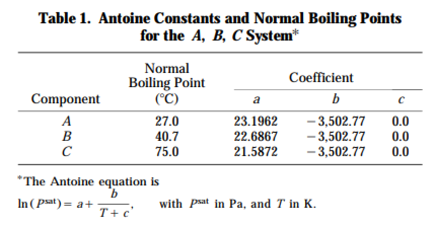
Vapor Pressure of components A, B and C

In[]:=

a1=23.1962;a2=22.6867;a3=21.5872;b1=-3502.77;b2=-3502.77;b3=-3502.77;c1=0;c2=0;c3=0;Psat[1]=Exp[a1+b1/(c1+T)];Psat[2]=Exp[a2+b2/(c2+T)];Psat[3]=Exp[a3+b3/(c3+T)];

Total Pressure

In[]:=

P=1.0132510^5;

Raoult’s law

In[]:=

y1=Psat[1]x1/P;y2=Psat[2]x2/P;y3=Psat[3]x3/P;

Summation rule

In[]:=

x3=1-x1-x2;

Equilibrium constant for the reaction A + B ⇄ C

In[]:=

Keq=5;

Computing the Jacobian Matrix

In[]:=

MYGrad[fon_,var_List]:=D[fon,#]&/@var

In[]:=

F[x1_,x2_,T_]:={(1-Dd)(x1-y1)+Dd(-1+x1)(x1x2-x3/Keq),(1-Dd)(x2-y2)+Dd(-1+x2)(x1x2-x3/Keq),1-Psat[1]x1/P-Psat[2]x2/P-Psat[3]x3/P}

In[]:=

M=MYGrad[F[x1,x2,T],{x1,x2,T}]

Out[]=

0.981-9.86923×

-6

23.1962-

3502.77



+0.02(-1+x1)

+x2+0.02x1x2+

(-1+x1+x2),0.02(-1+x2)

+x2,9.86923×

-6

21.5872-

3502.77



-9.86923×

-6

23.1962-

3502.77



,0.02(-1+x1)

+x1,0.981-9.86923×

-6

22.6867-

3502.77



+0.02

+x1(-1+x2)+0.02x1x2+

(-1+x1+x2),9.86923×

-6

21.5872-

3502.77



-9.86923×

-6

22.6867-

3502.77



,-

0.0338783

23.1962-

3502.77



0.0338783

22.6867-

3502.77



0.0345697

23.1962-

3502.77



0.0345697

21.5872-

3502.77



(1-x1-x2)

0.0345697

22.6867-

3502.77





Computing Branch 4

In[]:=

Dd=0.;i=0

Out[]=

In[]:=

sol[0]=FindRoot[{(1-Dd)(x1-y1)+Dd(-1+x1)(x1x2-x3/Keq)0,(1-Dd)(x2-y2)+Dd(-1+x2)(x1x2-x3/Keq)0,Psat[1]x1/P+Psat[2]x2/P+Psat[3]x3/P1},{x1,0.0},{x2,0.1},{T,320.0}]//Chop

Out[]=

{x10,x20,T348.149}

In[]:=

i=1;While[i<101,{Dd=0.01*i,sol[i]=FindRoot[{(1-Dd)(x1-y1)+Dd(-1+x1)(x1x2-x3/Keq)0,(1-Dd)(x2-y2)+Dd(-1+x2)(x1x2-x3/Keq)0,Psat[1]x1/P+Psat[2]x2/P+Psat[3]x3/P1},{x1,x1/.sol[i-1]},{x2,x2/.sol[i-1]},{T,T/.sol[i-1]},AccuracyGoal5],j=0,For[k=1,k≤3,k++,If[Re[(Eigenvalues[M][[k]]/.sol[i])]<0,j=j+1]],test=If[j3,"stable",If[j2,"saddle","unstable"]],Print[i," ",sol[i],Dd," ",Eigenvalues[M]/.sol[i]," ",test," ",j],i++}]

1 {x10.000506861,x20.00101233,T348.009}0.01 {-3.90617,-1.95881,-0.0287602} stable 3

2 {x10.00102723,x20.00205272,T347.866}0.02 {-3.88612,-1.9468,-0.0286183} stable 3

3 {x10.00156164,x20.00312231,T347.72}0.03 {-3.86568,-1.93456,-0.028473} stable 3

4 {x10.00211064,x20.0042223,T347.571}0.04 {-3.84485,-1.92208,-0.0283241} stable 3

5 {x10.00267482,x20.00535397,T347.418}0.05 {-3.82362,-1.90937,-0.0281716} stable 3

6 {x10.00325477,x20.00651866,T347.261}0.06 {-3.80198,-1.89641,-0.0280152} stable 3

7 {x10.00385114,x20.00771778,T347.101}0.07 {-3.77992,-1.8832,-0.0278548} stable 3

8 {x10.0044646,x20.00895281,T346.937}0.08 {-3.75743,-1.86973,-0.0276904} stable 3

9 {x10.00509587,x20.0102253,T346.769}0.09 {-3.73449,-1.85599,-0.0275217} stable 3

10 {x10.00574569,x20.011537,T346.598}0.1 {-3.71109,-1.84198,-0.0273485} stable 3

11 {x10.00641483,x20.0128896,T346.422}0.11 {-3.68722,-1.82769,-0.0271706} stable 3

12 {x10.00710413,x20.0142849,T346.241}0.12 {-3.66288,-1.81311,-0.026988} stable 3

13 {x10.00781446,x20.015725,T346.057}0.13 {-3.63803,-1.79824,-0.0268003} stable 3

14 {x10.00854672,x20.0172118,T345.867}0.14 {-3.61268,-1.78306,-0.0266074} stable 3

15 {x10.00930189,x20.0187476,T345.673}0.15 {-3.58681,-1.76758,-0.0264091} stable 3

16 {x10.010081,x20.0203347,T345.474}0.16 {-3.5604,-1.75177,-0.026205} stable 3

17 {x10.0108851,x20.0219757,T345.27}0.17 {-3.53345,-1.73563,-0.025995} stable 3

18 {x10.0117152,x20.0236729,T345.061}0.18 {-3.50593,-1.71916,-0.0257788} stable 3

19 {x10.0125727,x20.0254294,T344.846}0.19 {-3.47783,-1.70234,-0.025556} stable 3

20 {x10.0134588,x20.0272479,T344.625}0.2 {-3.44914,-1.68517,-0.0253265} stable 3

21 {x10.0143747,x20.0291316,T344.398}0.21 {-3.41984,-1.66763,-0.0250899} stable 3

22 {x10.0153218,x20.0310837,T344.166}0.22 {-3.38991,-1.64973,-0.0248459} stable 3

23 {x10.0163017,x20.0331079,T343.927}0.23 {-3.35935,-1.63144,-0.0245941} stable 3

24 {x10.0173158,x20.0352077,T343.682}0.24 {-3.32813,-1.61276,-0.0243341} stable 3

25 {x10.0183658,x20.0373872,T343.429}0.25 {-3.29625,-1.59368,-0.0240655} stable 3

26 {x10.0194534,x20.0396504,T343.17}0.26 {-3.26368,-1.5742,-0.0237879} stable 3

27 {x10.0205803,x20.0420019,T342.904}0.27 {-3.23041,-1.5543,-0.0235009} stable 3

28 {x10.0217483,x20.0444463,T342.63}0.28 {-3.19642,-1.53397,-0.023204} stable 3

29 {x10.0229596,x20.0469886,T342.348}0.29 {-3.16171,-1.51321,-0.0228966} stable 3

30 {x10.024216,x20.049634,T342.058}0.3 {-3.12626,-1.49201,-0.0225782} stable 3

31 {x10.0255197,x20.0523881,T341.76}0.31 {-3.09006,-1.47036,-0.0222483} stable 3

32 {x10.026873,x20.0552568,T341.454}0.32 {-3.05309,-1.44826,-0.0219062} stable 3

33 {x10.0282781,x20.0582463,T341.139}0.33 {-3.01534,-1.42569,-0.0215512} stable 3

34 {x10.0297373,x20.0613631,T340.814}0.34 {-2.97682,-1.40267,-0.0211827} stable 3

35 {x10.0312531,x20.0646139,T340.481}0.35 {-2.9375,-1.37917,-0.0207999} stable 3

36 {x10.0328279,x20.0680061,T340.137}0.36 {-2.89739,-1.35521,-0.0204021} stable 3

37 {x10.0344643,x20.0715471,T339.784}0.37 {-2.85649,-1.33077,-0.0199883} stable 3

38 {x10.0361647,x20.0752446,T339.421}0.38 {-2.8148,-1.30587,-0.0195577} stable 3

39 {x10.0379317,x20.0791067,T339.048}0.39 {-2.77233,-1.28051,-0.0191094} stable 3

40 {x10.0397677,x20.0831417,T338.664}0.4 {-2.72908,-1.25468,-0.0186423} stable 3

41 {x10.0416751,x20.087358,T338.27}0.41 {-2.68508,-1.22842,-0.0181555} stable 3

42 {x10.043656,x20.0917642,T337.866}0.42 {-2.64034,-1.20172,-0.0176477} stable 3

43 {x10.0457124,x20.0963688,T337.45}0.43 {-2.59489,-1.17461,-0.017118} stable 3

44 {x10.0478462,x20.10118,T337.024}0.44 {-2.54877,-1.14711,-0.016565} stable 3

45 {x10.0500586,x20.106207,T336.588}0.45 {-2.50202,-1.11924,-0.0159875} stable 3

46 {x10.0523506,x20.111456,T336.141}0.46 {-2.4547,-1.09104,-0.0153843} stable 3

47 {x10.0547226,x20.116936,T335.684}0.47 {-2.40687,-1.06255,-0.014754} stable 3

48 {x10.0571742,x20.122652,T335.218}0.48 {-2.35859,-1.03381,-0.0140954} stable 3

49 {x10.0597044,x20.128609,T334.743}0.49 {-2.30996,-1.00487,-0.0134072} stable 3

50 {x10.0623113,x20.134812,T334.259}0.5 {-2.26106,-0.975793,-0.0126879} stable 3

51 {x10.0649919,x20.141263,T333.767}0.51 {-2.212,-0.946637,-0.0119365} stable 3

52 {x10.0677421,x20.147962,T333.268}0.52 {-2.16288,-0.917473,-0.0111516} stable 3

53 {x10.0705566,x20.154907,T332.764}0.53 {-2.11385,-0.888377,-0.0103324} stable 3

54 {x10.073429,x20.162093,T332.255}0.54 {-2.06501,-0.859428,-0.00947764} stable 3

55 {x10.0763515,x20.169514,T331.743}0.55 {-2.01652,-0.830709,-0.0085867} stable 3

56 {x10.079315,x20.17716,T331.229}0.56 {-1.9685,-0.802307,-0.00765893} stable 3

Computing Branch 3

Computing Branch 1

Computing Branch 2A

Computing Branch 2B

Chemical equilibrium curve

Analysis of Simple Distillation: Case of a Hypothetical Ternary Mixture with Chemical Reaction​​ Authors: Housam Binous and Ahmed Bellagi

Analysis of Simple Distillation: Case of a Hypothetical Ternary Mixture with Chemical Reaction
Authors: Housam Binous and Ahmed Bellagi