This notebook solves a single-stage (isothermal) equilibrium flash for a binary liquid mixture, following the worked example in J. Benitez, Principles and Modern Applications of Mass Transfer Operations (Wiley-Interscience, 2002).
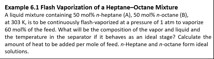
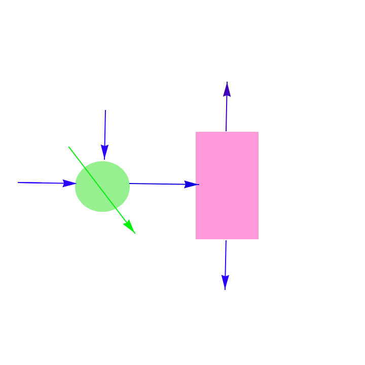
System: an equimolar (z = 0.5) liquid feed of components 1 and 2 (n-heptane and n-octane) enters a flash drum at atmospheric pressure P = 101.325 kPa.
A fraction ϕ of the feed is vaporized; the emerging vapor (mole fraction y) and liquid (mole fraction x) leave in equilibrium at temperature T.
A fraction ϕ of the feed is vaporized; the emerging vapor (mole fraction y) and liquid (mole fraction x) leave in equilibrium at temperature T.
Governing equations:
• Vapor pressures Psat1(T), Psat2(T) from Wagner equation for each pure component.
• Raoult’s-law equilibrium: y == K1 x and 1-y == K2 (1-x), with Ki == Psati(T)/P.
• Operating-line/material balance linking x, y and ϕ: (ϕ-1)/ϕ == (y-0.5)/(x-0.5).
• An energy balance (HD, HW, HF, Q) gives the heat added at the fixed operating point ϕ = 0.6.
1. Benitez example for ϕ=0.6
Notebook solves the three flash equations with FindRoot for one fixed vapor fraction, reproduces the textbook results for x, y and T, and evaluates the enthalpy balance.
Notebook solves the three flash equations with FindRoot for one fixed vapor fraction, reproduces the textbook results for x, y and T, and evaluates the enthalpy balance.
2. Arc-Length Continuation in ϕ
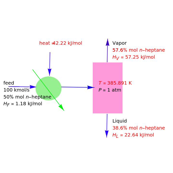
Code sweeps ϕ continuously from about 0 to 1 using pseudo arc-length continuation (rather than solving point by point) and plots how T, x and y evolve along the way.
Code sweeps ϕ continuously from about 0 to 1 using pseudo arc-length continuation (rather than solving point by point) and plots how T, x and y evolve along the way.
Benitez example for ϕ=0.6
Benitez example for ϕ=0.6
In[]:=
ϕ=0.6;(*vaporfraction*)
Psat[1]=27.4Exp-7.6751-+1.371-3.536-3.202;Psat[2]=24.9Exp-7.9121-+1.380-3.804-4.501;
1
1-1-
T
540.3
T
540.3
1.5
1-
T
540.3
3
1-
T
540.3
6
1-
T
540.3
1
1-1-
T
568.8
T
568.8
1.5
1-
T
568.8
3
1-
T
568.8
6
1-
T
568.8
In[]:=
K1=Psat[1]/P;K2=Psat[2]/P;
In[]:=
P=1.01325;
In[]:=
sol=FindRootyK1x,1-yK2(1-x),,{x,0.2},{y,0.4},{T,380};
ϕ-1
ϕ
y-0.5
x-0.5
In[]:=
HD=((y/.sol)187+(1-y/.sol)247)((T/.sol)-298)/1000+(y/.sol)36.5+(1-(y/.sol))41.4;HF=1.18;HW=((x/.sol)241+(1-x/.sol)268)((T/.sol)-298)/1000;Q=ϕHD+(1-ϕ)HW-HF;
In[]:=
Q
Out[]=
42.2238
Show
,Graphics
Out[]=
Arc-Length Continuation in ϕ
Arc-Length Continuation in ϕ
This section re-solves the flash equations above while treating ϕ itself as a free continuation parameter, using pseudo arc-length continuation. Instead of stepping ϕ directly (which can stall near turning points and requires good initial guesses), each step advances along the solution curve {x,y,T,ϕ} by a fixed arc-length ds: a tangent-line predictor followed by a Newton corrector that solves the physical equations together with an arc-length constraint.
The operating-line equation is rearranged to (ϕ-1)(x-0.5)==ϕ(y-0.5) so it stays regular at ϕ=0.
The operating-line equation is rearranged to (ϕ-1)(x-0.5)==ϕ(y-0.5) so it stays regular at ϕ=0.
In[]:=
Clear[ϕ]F1[xx_,yy_,TT_]:=yy-(K1/.T->TT)xxF2[xx_,yy_,TT_]:=(1-yy)-(K2/.T->TT)(1-xx)F3[xx_,yy_,ph_]:=(ph-1)(xx-0.5)-ph(yy-0.5)Fres[{xx_,yy_,TT_,ph_}]:=N[{F1[xx,yy,TT],F2[xx,yy,TT],F3[xx,yy,ph]}]
JacNumeric[u_List]:=Module[{eps=1.*^-6},Transpose@Table[(Fres[ReplacePart[u,i->u[[i]]+eps]]-Fres[ReplacePart[u,i->u[[i]]-eps]])/(2eps),{i,4}]]Tangent[u_List,tPrev_:None]:=Module[{ns,t},ns=NullSpace[JacNumeric[u]];If[ns==={},Return[$Failed]];t=First[ns];t=t/Norm[t];If[tPrev=!=None&&t.tPrev<0,t=-t];t]
In[]:=
Corrector[u0_List,t0_List,ds_]:=Module[{pred=u0+dst0,sol},sol=Quiet@Check[FindRoot[{F1[x,y,T]==0,F2[x,y,T]==0,F3[x,y,ϕ]==0,t0.({x,y,T,ϕ}-u0)-ds==0},{{x,pred[[1]]},{y,pred[[2]]},{T,pred[[3]]},{ϕ,pred[[4]]}},MaxIterations->200],$Failed];If[sol===$Failed,$Failed,{x,y,T,ϕ}/.sol]]
In[]:=
RunBranch[u0_List,t0Init_List,ds0_,nSteps_,dir_:1]:=Module[{u=u0,t=dirt0Init,ds=ds0,path={},unew,tnew,fails=0},Do[unew=Corrector[u,t,ds];If[unew===$Failed,ds=ds/2;fails++;If[ds<1.*^-5||fails>12,Break[]],If[unew[[4]]<-0.02||unew[[4]]>1.02||unew[[1]]<-0.05||unew[[1]]>1.05||unew[[2]]<-0.05||unew[[2]]>1.05,Break[]];tnew=Tangent[unew,t];If[tnew===$Failed,Break[]];u=unew;t=tnew;ds=ds0;fails=0;AppendTo[path,u]],{nSteps}];path]
Starting point: the ϕ=0.6 flash solved earlier in the notebook
u0=Append[{x,y,T}/.sol,0.6];t0=Tangent[u0];branchUp=RunBranch[u0,t0,0.01,500,0.01];branchDown=RunBranch[u0,t0,0.01,500,-0.01];continuationPath=SortBy[Join[Reverse[branchDown],{u0},branchUp],Last];Length[continuationPath]
Out[]=
351
In[]:=
phiVals=continuationPath[[All,4]];xVals=continuationPath[[All,1]];yVals=continuationPath[[All,2]];TVals=continuationPath[[All,3]];flashContinuationData=Transpose[{phiVals,xVals,yVals,TVals}];
RowListLinePlotTranspose[{phiVals,TVals}],," ",ListLinePlot{Transpose[{phiVals,xVals}],Transpose[{phiVals,yVals}]},
CITE THIS NOTEBOOK
CITE THIS NOTEBOOK
Single-stage flash distillation of a binary mixture: equilibrium solution and continuation in φ
by Housam Binous
Wolfram Community, STAFF PICKS, September 20, 2026
https://community.wolfram.com/t/28095/1
by Housam Binous
Wolfram Community, STAFF PICKS, September 20, 2026
https://community.wolfram.com/t/28095/1