PascalTheorem::usage=" In any hexagon inscribed in a conical section, the continuations of opposite sides meet on a straight line, called the Pascal line. This property is repeated in Geometry, there is also the Monge's theorem and the Desargues' theorem. References: Personal, based in the Pascal's theorem. ";
Development:
Obtaining the vertices of the hexagon in numerical form:
In[]:=
r=2;k=2;d=1;n=6;ρ=;x1=4;y1=6;Table{4-d,y1}++-{(r+ρ)Cos[t1]+x1-(4-d),(r+ρ)Sin[t1]+y1-6},t1,0,2π,
2Sin
π
n
1-Sin
π
n
2
k
2
((r+ρ)Cos[t1]+x1-(4-d))
2
((r+ρ)Sin[t1]+y1-6)
2
ρ
2π
n
,6,,6+,,6+,,6,,6-,,6-,,6;
83
21
63
17
8
3
17
23
9
8
3
3
3
5
23
9
8
3
3
63
17
8
3
17
83
21
In[]:=
Showr=2;k=2;d=1;n=6;ρ=;x1=4;y1=6;GraphicsRed,PointSize[0.015],Point,6,GraphicsBlue,PointSize[0.015],Point,6+,GraphicsGreen,PointSize[0.015],Point,6+,GraphicsGray,PointSize[0.015],Point,6,GraphicsPink,PointSize[0.015],Point,6-,GraphicsPurple,PointSize[0.015],Point,6-,ParametricPlotCos[θ]+,Sin[θ]+6,{θ,0,2π},ColorFunction->"DarkRainbow",TableGraphicsDarkGreen,Thick,Line{4-d,y1}++-{(r+ρ)Cos[t1]+x1-(4-d),(r+ρ)Sin[t1]+y1-6},{4-d,y1}++-(r+ρ)Cost1++x1-(4-d),(r+ρ)Sint1++y1-6,t1,0,2π,,TableGraphicsBlack,Thick,Dashed,InfiniteLine{4-d,y1}++-{(r+ρ)Cos[t1]+x1-(4-d),(r+ρ)Sin[t1]+y1-6},{4-d,y1}++-(r+ρ)Cost1++x1-(4-d),(r+ρ)Sint1++y1-6,t1,0,2π,,AxesTrue,BoxRatiosAutomatic,AxesOrigin{0,0},ImageSize700,PlotRange{{0,10},{0,10}}
2Sin
π
n
1-Sin
π
n
83
21
63
17
8
3
17
23
9
8
3
3
3
5
23
9
8
3
3
63
17
8
3
17
176
105
239
105
16
105
2
k
2
((r+ρ)Cos[t1]+x1-(4-d))
2
((r+ρ)Sin[t1]+y1-6)
2
ρ
2
k
2
(r+ρ)Cost1++x1-(4-d)
2π
n
2
(r+ρ)Sint1++y1-6
2π
n
2
ρ
2π
n
2π
n
2π
n
2
k
2
((r+ρ)Cos[t1]+x1-(4-d))
2
((r+ρ)Sin[t1]+y1-6)
2
ρ
2
k
2
(r+ρ)Cost1++x1-(4-d)
2π
n
2
(r+ρ)Sint1++y1-6
2π
n
2
ρ
2π
n
2π
n
2π
n
Out[]=
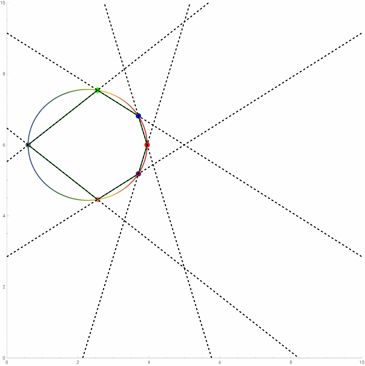
Obtaining the equations of the opposite sides:
GrayGreen line and PurpleRedline, form the point 1:
In[]:=
Solve(y-6)-==6+-6x-,y-6--==6-6-x-,{x,y}
23
9
3
5
8
3
3
3
5
8
3
17
83
21
63
17
8
3
17
63
17
x5,y23+
3
;GreenBlue line and PinkPurple, form the point 2:
In[]:=
Solvey-6+-==6+-6+x-,y-6--==6--6-x-,{x,y}
8
3
3
63
17
23
9
8
3
17
8
3
3
23
9
8
3
3
63
17
23
9
8
3
17
8
3
3
23
9
{{x5,y6}};
GrayPink line and BlueRed line, form the point 3:
In[]:=
Solve(y-6)-==6--6x-,y-6+-==6-6+x-,{x,y}
23
9
3
5
8
3
3
3
5
8
3
17
83
21
63
17
8
3
17
63
17
x5,y-2-3+
3
;Complete graph:
In[]:=
Showr=2;k=2;d=1;n=6;ρ=;x1=4;y1=6;GraphicsRed,PointSize[0.015],Point,6,GraphicsBlue,PointSize[0.015],Point,6+,GraphicsGreen,PointSize[0.015],Point,6+,GraphicsGray,PointSize[0.015],Point,6,GraphicsPink,PointSize[0.015],Point,6-,GraphicsPurple,PointSize[0.015],Point,6-,Graphics[Black,PointSize[0.015],Point[5,23+Cos[θ]+,Sin[θ]+6,{θ,0,2π},ColorFunction->"DarkRainbow",TableGraphicsDarkGreen,Thick,Line{4-d,y1}++-{(r+ρ)Cos[t1]+x1-(4-d),(r+ρ)Sin[t1]+y1-6},{4-d,y1}++-(r+ρ)Cost1++x1-(4-d),(r+ρ)Sint1++y1-6,t1,0,2π,,TableGraphicsBlack,Thick,Dashed,InfiniteLine{4-d,y1}++-{(r+ρ)Cos[t1]+x1-(4-d),(r+ρ)Sin[t1]+y1-6},{4-d,y1}++-(r+ρ)Cost1++x1-(4-d),(r+ρ)Sint1++y1-6,t1,0,2π,,AxesTrue,BoxRatiosAutomatic,AxesOrigin{0,0},ImageSize700,PlotRange{{0,10},{0,10}}
2Sin
π
n
1-Sin
π
n
83
21
63
17
8
3
17
23
9
8
3
3
3
5
23
9
8
3
3
63
17
8
3
17
3
]],Graphics[{Black,PointSize[0.015],Point[{5,6}]}],Graphics[Black,PointSize[0.015],Point[5,-2-3+3
]],Graphics[Black,Thick,InfiniteLine[{5,6},5,-2-3+3
]],ParametricPlot176
105
239
105
16
105
2
k
2
((r+ρ)Cos[t1]+x1-(4-d))
2
((r+ρ)Sin[t1]+y1-6)
2
ρ
2
k
2
(r+ρ)Cost1++x1-(4-d)
2π
n
2
(r+ρ)Sint1++y1-6
2π
n
2
ρ
2π
n
2π
n
2π
n
2
k
2
((r+ρ)Cos[t1]+x1-(4-d))
2
((r+ρ)Sin[t1]+y1-6)
2
ρ
2
k
2
(r+ρ)Cost1++x1-(4-d)
2π
n
2
(r+ρ)Sint1++y1-6
2π
n
2
ρ
2π
n
2π
n
2π
n
The graph shows Pascal’s line.