Petri nets are directed bipartite graphs useful to model discrete dynamical systems. We explore, following their number of nodes and edges, different Petri nets and compute their evolution over time. Finally, we propose a Petri net classification based on the mean distribution of tokens over time, and search for the emergence of complex behavior.
Introduction
Introduction
In “A New Kind of Science”, Stephen Wolfram explores the emergence of complex behavior from simple rules for cellular automata . Following this idea, we compute every possible Petri nets in order of number of components, and evolved them in time. We find the appearance of clusters for the evolution of the total number of tokens, which provide us with a systematic method to classify our nets and a way to observe the emergence of complexity as we increase the number of components.
Petri Nets
Petri Nets
A Petri net is composed by two different kinds of nodes: places and transitions. Places contain tokens, and the distribution of tokens in different places represent the current state of the system, also known as marking. Transitions are the possible events to occur, given that the marking accomplishes certain conditions. Finally our nodes and transitions are connected by directed edges which show how different places interact through transitions.
To generate all possible petri nets given the number of elements, first we label places with Alphabet[], transitions with Alphabet["Greek"] and generate a list of all possible edges. For instance :
To generate all possible petri nets given the number of elements, first we label places with Alphabet[], transitions with Alphabet["Greek"] and generate a list of all possible edges. For instance :
In[]:=
numberofPlaces=2;numberofTransitions=2;numberofEdges=2;markingInitialperPlace=6;
In[]:=
places=Alphabet[]〚1;;numberofPlaces〛transitions=Alphabet["Greek"]〚1;;numberofTransitions〛listofEdges=Sort[DeleteDuplicates[Sort/@Tuples[Flatten[Table[{ij,ji},{i,places},{j,transitions}]],numberofEdges]]]markingInitial=Table[markingInitialperPlace,numberofPlaces]
Out[]=
{a,b}
Out[]=
{α,β}
Out[]=
{{aα,aα},{aα,aβ},{aα,bα},{aα,bβ},{aα,αa},{aα,αb},{aα,βa},{aα,βb},{aβ,aβ},{aβ,bα},{aβ,bβ},{aβ,αa},{aβ,αb},{aβ,βa},{aβ,βb},{bα,bα},{bα,bβ},{bα,αa},{bα,αb},{bα,βa},{bα,βb},{bβ,bβ},{bβ,αa},{bβ,αb},{bβ,βa},{bβ,βb},{αa,αa},{αa,αb},{αa,βa},{αa,βb},{αb,αb},{αb,βa},{αb,βb},{βa,βa},{βa,βb},{βb,βb}}
Out[]=
{6,6}
We compute a step in the network dynamics with evolutionStep. For example, for a previous Petri net with edge {“b””β”,”β””a”} we have two possibilities, or “α” is fired and the marking does not change, or “β” fires and we diminish the number of tokens of “b” by 1 and increase the ones in “a” by 1. This transition is chosen randomly:
evolutionStep[places,transitions,{"b""β","β""a"},markingInitial]
Out[]=
{7,5}
We see, in this example “β” was fired an therefore, we have 7 tokens in “a” and 5 in “b”.
We iterate evolutionStep in order to have multistep evaluations. In the following example we use a step of 1, starting from 0 to 10. Also, we set a numberofIterations to compute a mean and a standard deviation of our tokens so we can take into account the stochasticity of our Petri net.
In[]:=
numberofIterations=100;
In[]:=
marking=N[evolutionList[places,transitions,{"b""β","β""a"},markingInitial,1,0,10]]
Out[]=
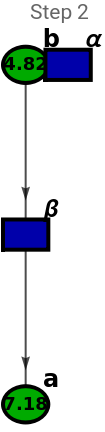
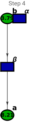
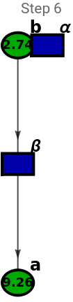
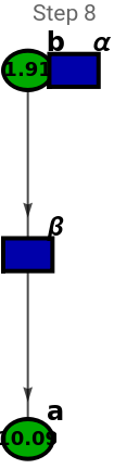
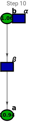
{{6.±0.,6.±0.},{6.65±0.479372,5.35±0.479372},{7.18±0.6724,4.82±0.6724},{7.66±0.890125,4.34±0.890125},{8.21±1.02784,3.79±1.02784},{8.72±1.11988,3.28±1.11988},{9.26±1.19443,2.74±1.19443},{9.74±1.2762,2.26±1.2762},{10.09±1.28782,1.91±1.28782},{10.58±1.21589,1.42±1.21589},{10.94±1.14433,1.06±1.14433}}
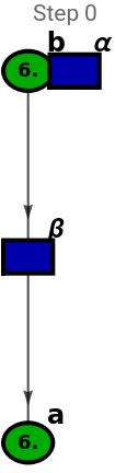
For visualization, we prepare the function petriNetPlot which plots the structure of our petri net, where places are green ellipses and transitions blue rectangles:
In[]:=
Table[petriNetPlot[places,transitions,{"b""β","β""a"},marking〚i〛〚All,1〛,"Step "<>ToString[i-1]],{i,1,11,2}]
Out[]=
,
,
,
,
,
Also, to get a better insight of the net, we compute its respective Incidence Matrix, which shows how tokens in a place change as an specific transition fires.
In[]:=
incidenceMatrix[places,transitions,{"b""β","β""a"}]//MatrixForm
Out[]//MatrixForm=
0 | 1 |
0 | -1 |
Simple Petri Nets
Simple Petri Nets
Following Stephen’s idea, we find an analog to the cellular automata system:
In[]:=
Grid[{{"Cellular Automata"," ","Petri Nets"},{"State","","Marking"},{"Rules","","Topology of the net (places, transitions and edges)"}},Spacings{1,2},FrameAll,FrameStyleDirective[Gray,Opacity[0.2]],Background{None,{1RGBColor[0.5,0.5,0.5,0.3]}}]
Out[]=
Cellular Automata | Petri Nets | |
State | | Marking |
Rules | | Topology of the net (places, transitions and edges) |
We start working with Petri nets with small amounts of places, transitions and edges. We come up with a function petriNetStudy which, given the number of positions, transition, edges and tokens in each place, compute every possible petri net following this characteristics, together with its evolution in time.
In[]:=
TableForm[N[petriNetStudy[1,2,1,6]]]
Out[]//TableForm=
a | |||||||||||||||||||||||||||||||||||||||||||||||
α | β | ||||||||||||||||||||||||||||||||||||||||||||||
|
|
|
| ||||||||||||||||||||||||||||||||||||||||||||
6. | |||||||||||||||||||||||||||||||||||||||||||||||
|
|
|
|
In this example we use one position labeled by "a", two transitions "α" and "β", one edge and six tokens in "a". We observe that there are four possible petri nets with these characteristics, and also the evolution of the number of tokens in "a". Note the error in this number, product of the stochastic nature when choosing to fire "α" or "β".
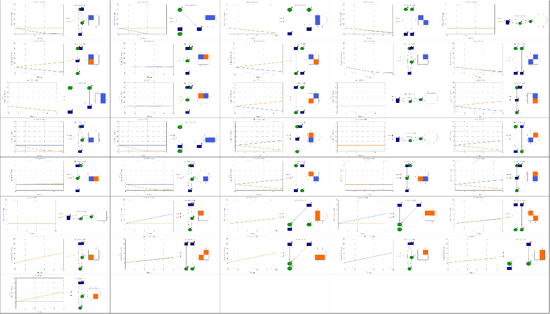
To make interpretation easier, we implement plotStudy to plot the number of tokens vs time, the petri net structure and its respective incidence matrix.
plotStudy[petriNetStudy[1,2,1,6]]

For a more interesting set of parameters:
plotStudy[petriNetStudy[2,2,2,6]]
We use FeatureSpacePlot to search for common dynamics in the tokens. We find:
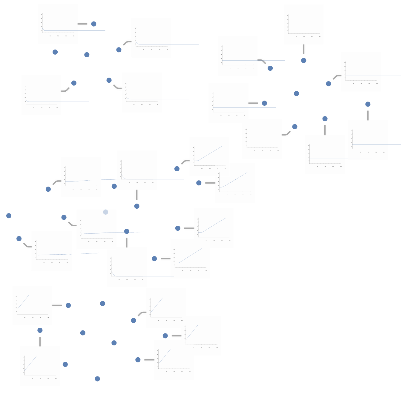
Where we observe 5 different evolutions:
We also identify the emergence of new classes as we increases the values of our parameters. For example, for 3 places, transitions an edges we have:
Were we find this other class:
Finally, we can also map this classification into the structure of the net, or the incidence matrix:
Now, we are ready to explore a bigger parameter space, and search for the emergence of a complex number of tokens dynamics. For now, this is our main future direction.
Future Directions
Future Directions
◼
Data for many different parameters has been computed, however, due to computational power limitations only a subset of that dataset was analyzed. Exploring a larger parameter space to observe the emergence of complex token dynamics behavior is an immediate future goal.
◼
Optimize or code, modding over label symmetries.
◼
Find possible relations between or classification and invariants of the incidence matrix, as singular values, the permanents, etc.
References
References
◼
Wolfram, Stephen. A New Kind of Science. Champaign, IL: Wolfram Media, 2002. Print.
◼
Implement Petri net by Pumeng Lyu, University of Wisconsin Madison. https://community.wolfram.com/groups/-/m/t/1728556
◼
Reisig, W.. (2013). Understanding Petri nets. Modeling techniques, analysis methods, case studies.