Improved Supply and Demand Curves

Ordinary supply and demand graphs that I was taught in school involve two linear forces and their intersection.
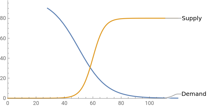
This more detailed supply and demand graph incorporates the concept of saturation.
In this model, supply & demand have limits and non-linear rates of change.

In[]:=

(*Definefunctionsfordemandandsupply*)demand[maxDemand_,rateChangeDemand_,price_,priceAtHalfMaxDemand_]:=maxDemand/(1+Exp[-rateChangeDemand*(price-priceAtHalfMaxDemand)]);supply[maxSupply_,rateChangeSupply_,price_,priceAtHalfMaxSupply_]:=maxSupply/(1+Exp[-rateChangeSupply*(price-priceAtHalfMaxSupply)]);(*Setparametervalues(adjusttheseasneeded)*)maxDemand=100;rateChangeDemand=-0.1;priceAtHalfMaxDemand=50;maxSupply=80;rateChangeSupply=.25;priceAtHalfMaxSupply=60;(*Definepricerangeforthegraph*)priceRange={0,120};(*Generatedemandandsupplydatapoints*)demandPoints=Table[{price,demand[maxDemand,rateChangeDemand,price,priceAtHalfMaxDemand]},{price,priceRange[[1]],priceRange[[2]]}];supplyPoints=Table[{price,supply[maxSupply,rateChangeSupply,price,priceAtHalfMaxSupply]},{price,priceRange[[1]],priceRange[[2]]}];(*Createtheplot*)plot=Plot[{demand[maxDemand,rateChangeDemand,price,priceAtHalfMaxDemand],supply[maxSupply,rateChangeSupply,price,priceAtHalfMaxSupply]},{price,priceRange[[1]],priceRange[[2]]},PlotRange->{{0,maxDemand+10},{0,maxSupply+10}},PlotLabels->{"Demand","Supply"}];Show[plot]

Out[]=

In[]:=

(*Definefunctionfordifferencebetweendemandandsupply*)Difference[price_]:=demand[maxDemand,rateChangeDemand,price,priceAtHalfMaxDemand]-supply[maxSupply,rateChangeSupply,price,priceAtHalfMaxSupply];(*FindtheequilibriumpriceusingFindRoot*)equilibriumPrice=FindRoot[Difference,{price,60}](*Initialguessaround60*)(*Printtheequilibriumprice*)Print["Equilibrium price:",equilibriumPrice[[1,1]]]demand[maxDemand,rateChangeDemand,price,priceAtHalfMaxDemand]-supply[maxSupply,rateChangeSupply,price,priceAtHalfMaxSupply]

FindRoot

:The function value {Difference} is not a list of numbers with dimensions {1} at {price} = {60.}.

FindRoot

:The function value {Difference} is not a list of numbers with dimensions {1} at {price} = {60.}.

Out[]=

FindRoot[Difference,{price,60}]

FindRoot

:The function value {Difference} is not a list of numbers with dimensions {1} at {price} = {60.}.

Part

:Part specification FindRoot[Difference,{price,60}]〚1,1〛 is longer than depth of object.

Equilibrium price:FindRoot[Difference,{price,60}]〚1,1〛

Out[]=

-0.25(-60+price)



100Null

0.1(-50+price)



In[]:=

Solve-

-0.25`(-60+price)



100

0.1`(-50+price)



==0,price,Reals

Solve

:Solve was unable to solve the system with inexact coefficients. The answer was obtained by solving a corresponding exact system and numericizing the result.

Out[]=