In[]:=
ClearAll["`*"];
experimental data :
experimental data :
expo decay data:-
expo decay data:-
In[]:=
(*--------Importexperimentaldata--------------*)
In[]:=
rawExpData1=Import["D:\\RAJESH CHELL\\Data for TF Rajesh\\Gain100\\detectorNLPQT\\R23 CO line 5 Torr Gain 100 NLPQT\\CO_R23_5Torr_detektorNLPQT_gain100_tfit0us_ringdowns_01.csv","Data"][[17]];
ringdowny1=rawExpData1[[3;;]];(*1sttw0areheading,*)dt=0.04;t=Table[n*dt,{n,0,Length[ringdowny1]-1}];tlast=t[[-1]];fs=1/dt;
In[]:=
nSamples=Length[t]
Out[]=
5120
In[]:=
Length[t]
Out[]=
5120
In[]:=
rawExpData=Transpose[{t,ringdowny1}]
Out[]=
y1=ListPlot[Transpose[{t,ringdowny1}],PlotRange->All,Joined->True,Mesh->Full]
Out[]=

transfer function:-
transfer function:-
In[]:=
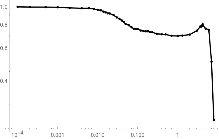
tdata=Import["D:\\RAJESH CHELL\\Data for TF Rajesh\\Gain100\\detectorNLPQT\\Pomiar nieliniowosci pasma detektora NLPQT_gain100_01.csv","Data"];freq=tdata[[2;;]][[All,2]];normTF=tdata[[2;;]][[All,8]];
In[]:=
magData=Delete[Delete[Transpose[{freq,normTF}],20],26];
In[]:=
t1=ListLogLogPlot[magData,PlotRange->All,Joined->True,Mesh->All,PlotStyle->Black]
Out[]=
exponential fitting :
exponential fitting :
fitting of whole Data:-
fitting of whole Data:-
In[]:=
fit1=NonlinearModelFit[rawExpData,a1*Exp[-time/tau1]+con1,{{a1,0.15},{tau1,32},{con1,0.003}},time,WorkingPrecision->16]

Out[]=
FittedModel
In[]:=
fit1["ParameterTable"]
Out[]=
Estimate | Standard Error | t-Statistic | P-Value | |
a1 | 0.1713690460156431 | 0.00012002125207318 | 1427.8225152255 | 2.04387845007× -6658 10 |
tau1 | 5.117045800481729 | 0.005227429980277 | 978.8836617207 | 1.19041498994× -5822 10 |
con1 | 0.006901500080689965 | 0.000010076818835140 | 684.8887723001 | 4.3891856010× -5035 10 |
In[]:=
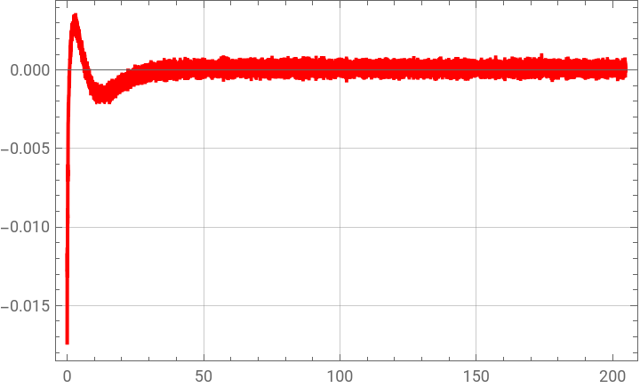
residual1=Transpose[{rawExpData[[All,1]],fit1["FitResiduals"]}];ListPlot[residual1,PlotRange->All,PlotStyle->Red,Frame->True,GridLines->Automatic,Joined->True]
Out[]=
fitting of selected Data:-
fitting of selected Data:-
In[]:=
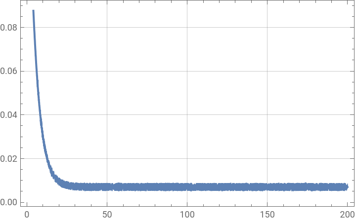
tStrt=4;tEnd=200;
In[]:=
selectedData=Select[rawExpData,tStrt<=#[[1]]<=tEnd&];
In[]:=
ListPlot[selectedData,PlotRange->All,Joined->True,Frame->True,GridLines->Automatic]
Out[]=
In[]:=
fit2=NonlinearModelFit[selectedData,a1*Exp[-time/tau1]+con1,{{a1,0.1},{tau1,32},{con1,0.02}},time,WorkingPrecision->15,Method->"LevenbergMarquardt"]
Out[]=
FittedModel
In[]:=
fit2["ParameterTable"]
Out[]=
Estimate | Standard Error | t-Statistic | P-Value | |
a1 | 0.191405924041317 | 0.0001471041131530 | 1301.159566097 | 7.077356594× -6223 10 |
tau1 | 4.69815288929730 | 0.002555100213660 | 1838.735273153 | 5.733616069× -6957 10 |
con1 | 0.00697433716427901 | 2.502830446931× -6 10 | 2786.579959034 | 1.9147496155× -7840 10 |
In[]:=
fittedParamValue2=Values[fit2["BestFitParameters"]];fittedParams2=Keys[fit2["BestFitParameters"]];std2=fit2["ParameterErrors"];
In[]:=
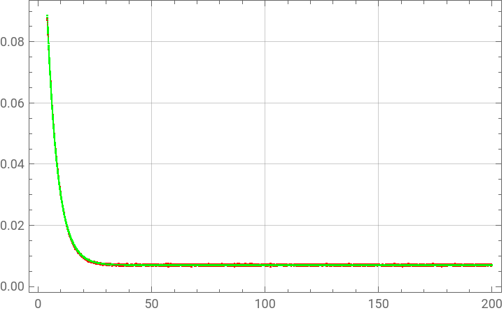
fittedData2=Table[{selectedData[[k,1]],fit2[selectedData[[k,1]]]},{k,1,Length[selectedData]}];
In[]:=
ListPlot[{selectedData(*wholeData*),fittedData2},Frame->True,GridLines->Automatic,Joined->{False,False},PlotRange->All,PlotStyle->{Red,Green},PlotLegends->{"selectedData","fittedData"}]
Out[]=


fitting using convolution:
fitting using convolution:
define convolution :-
define convolution :-
parameter list:-
parameter list:-
check with initial value:-
check with initial value:-
Fit:-
Fit:-
parameter Table
parameter Table
Residual plot
Residual plot
transfer function after convolution:-
transfer function after convolution:-