Conversion of Methanol to Formaldehyde
Authors: Housam Binous and Ahmed Bellagi
Conversion of Methanol to Formaldehyde
Authors: Housam Binous and Ahmed Bellagi
Authors: Housam Binous and Ahmed Bellagi
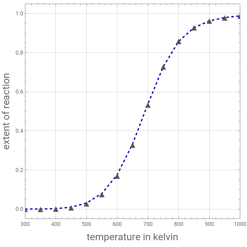
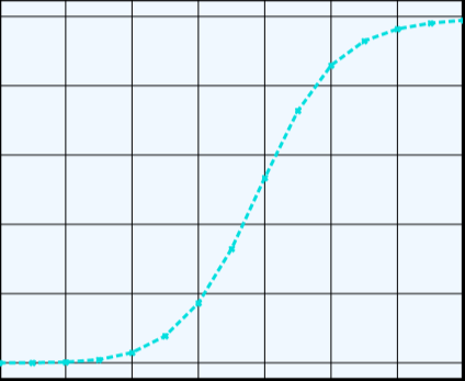
Consider the production of formaldehyde by gas-phase pyrolysis of methanol [Ref. 1] by the reaction OH(g)⇌O(g)+(g). Here, we plot the extent of the reaction versus temperature (in kelvin) for a pressure . Two methods are compared: (1) the Gibbs free energy minimization technique, shown by the gray triangles; and (2) the reaction coordinate method, indicated by the blue dashed curve. Perfect agreement is observed between the two approaches. Our results agree with their counterparts obtained using Aspen-HYSYS. You can check that Le Châtelier’s Principle is verified:
Low pressure (i.e., 1 atm) favors conversion to formaldehyde and hydrogen.
Increasing temperature shifts equilibrium toward products (formaldehyde + hydrogen).
References:
[1] M. D. Koretsky, Engineering and Chemical Thermodynamics, 2nd ed., Hoboken, NJ: Wiley, 2013.
CH
3
CH
2
H
2
P=1atm
Low pressure (i.e., 1 atm) favors conversion to formaldehyde and hydrogen.
Increasing temperature shifts equilibrium toward products (formaldehyde + hydrogen).
References:
[1] M. D. Koretsky, Engineering and Chemical Thermodynamics, 2nd ed., Hoboken, NJ: Wiley, 2013.
In[]:=
P1=1;R=8.314;Gj=10^3{{-272.667,-273.110,-297.819,-323.827,-351.028,-379.343,-408.711,-439.077,-470.388},{-181.126,-181.531,-203.980,-227.417,-251.733,-276.853,-302.722,-329.290,-356.516},{-38.962,-39.204,-52.727,-66.987,-81.836,-97.175,-112.937,-129.070,-145.536}};Te=Join[{298.15},Table[i,{i,300,1000,100}]];DataCH4O=Table[{Te[[i]],Gj[[1,i]]},{i,1,9}];solCH4O=FindFit[DataCH4O,a1+a2x+a3x^2+a4x^3+a5x^4+a6x^5+a7x^6+a8x^7+a9x^8+a10xLog[x],{a1,a2,a3,a4,a5,a6,a7,a8,a9,a10},x];DataCH2O=Table[{Te[[i]],Gj[[2,i]]},{i,1,9}];solCH2O=FindFit[DataCH2O,a1+a2x+a3x^2+a4x^3+a5x^4+a6x^5+a7x^6+a8x^7+a9x^8+a10xLog[x],{a1,a2,a3,a4,a5,a6,a7,a8,a9,a10},x];DataH2=Table[{Te[[i]],Gj[[3,i]]},{i,1,9}];solH2=FindFit[DataH2,a1+a2x+a3x^2+a4x^3+a5x^4+a6x^5+a7x^6+a8x^7+a9x^8+a10xLog[x],{a1,a2,a3,a4,a5,a6,a7,a8,a9,a10},x];K0=Exp[-52000/R/T0];K[T_]:=K0Exp[A[T]];T0=298.15;A[T_]:=(-84700/R+3.302T0-4.77610^-3/2T0^2+1.5710^-6/3T0^3-0.08310^5/298)(1/T-1/T0)+3.302Log[T/T0]-4.77610^-3/2(T-T0)+1.5710^-6/6(T^2-T0^2)+0.08310^5/2(1/T^2-1/T0^2);
In[]:=
P=1;(*pressureinatm*)
In[]:=
Gtot[x_,P_]:=Re[Sum[n[j]*(G[x,P,j]+RxLog[n[j]/Sum[n[k],{k,1,3}]]),{j,1,3}]];sol[T_,P_]:=Quiet@NMinimize[Flatten[{Gtot[T,P],Table[n[j]≥0,{j,1,3}],n[1]+n[2]==1.0,4n[1]+2n[2]+2n[3]==4}],{n[1],n[2],n[3]},MaxIterations10];G[x_,P_,1]:=((a1+a2x+a3x^2+a4x^3+a5x^4+a6x^5+a7x^6+a8x^7+a9x^8+a10xLog[x])/.solCH4O)+RxLog[P/P1];G[x_,P_,2]:=((a1+a2x+a3x^2+a4x^3+a5x^4+a6x^5+a7x^6+a8x^7+a9x^8+a10xLog[x])/.solCH2O)+RxLog[P/P1];G[x_,P_,3]:=((a1+a2x+a3x^2+a4x^3+a5x^4+a6x^5+a7x^6+a8x^7+a9x^8+a10xLog[x])/.solH2)+RxLog[P/P1];t1=Quiet@Table[{T,Quiet@n[2]/.sol[T,P][[2]]},{T,300,1000,50}];t2=Table[{T,xi/.FindRoot[K[T]Pxixi/(1-xi)/(1+xi),{xi,0.96}]},{T,300,1000,50}];p1=ListPlot[t1,FrameTrue,GridLinesAutomatic,AspectRatio1,PlotMarkers{Style["▲",Darker@Gray,16]},PlotRange{{300,1000},{-0.05,1.05}}];p2=ListPlot[t2,FrameTrue,GridLinesAutomatic,AspectRatio1,JoinedTrue,PlotStyle{Thick,Darker@Blue,Dashed},PlotRange{{300,1000},{-0.05,1.05}}];Show[p2,p1,FrameLabel{Style["temperature in kelvin",16],Style["extent of reaction",16]},ImageSize400{1,1},PlotRange{{300,1000},{-0.05,1.05}}]
Out[]=
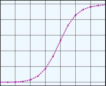
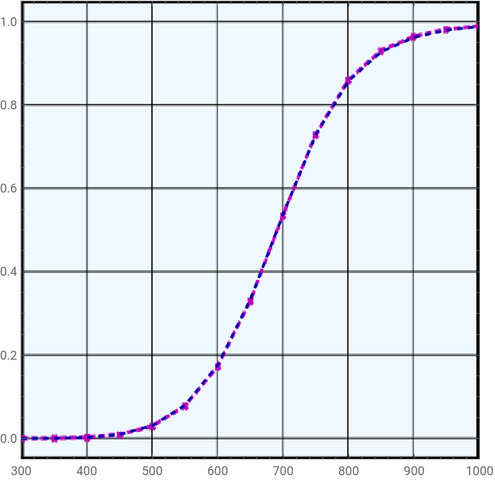
Comparison with Aspen - HYSYS (REquil in dashed magenta and RGibbs in dashed cyan)
In[]:=
img=
;
In[]:=
Show[p2,Prolog->{Raster[ImageData[img,DataReversed->True],{Scaled[{0.0,0.0}],Scaled[{1,1}]}]}]
Out[]=
In[]:=
img=
;
In[]:=
Show[p1,Prolog->{Raster[ImageData[img,DataReversed->True],{Scaled[{0.0,0.0}],Scaled[{1,1}]}]}]
Out[]=
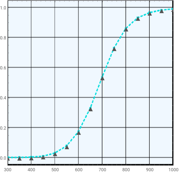
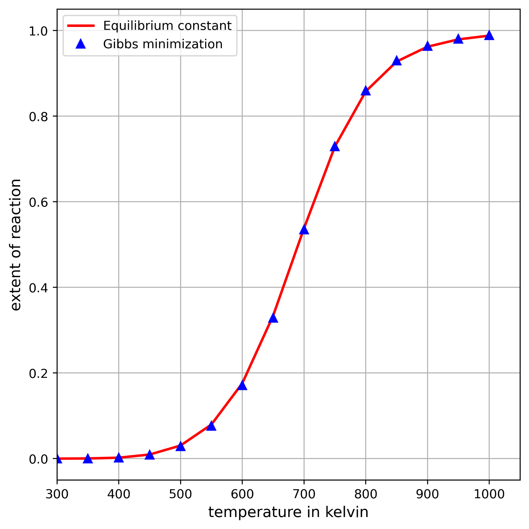
Asimilarresult,obtainedwithPython,isshownbelow(Pythoncodeisavailableuponrequest):