Introduction
Introduction
A new paper arrived on the ArXiv last week which has generated a lot of attention across social media: https://arxiv.org/pdf/2602.12176 (“Single-minus gluon tree amplitudes are nonzero”). Within the paper, the authors present various single-minus tree-level n-gluon stripped amplitudes before generalizing the result to arbitrary n > 2. In particular, the authors present the n = 3, 4, 5, and 6 stripped amplitudes in Eqs. 29-32:
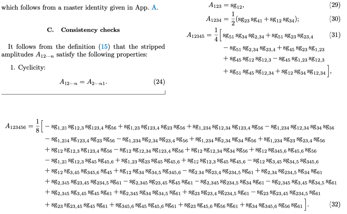
before remarking: “Clearly a more concise formula is needed!”, and indeed -- after further restricting the kinematic region, they report simpler expressions for these cases:
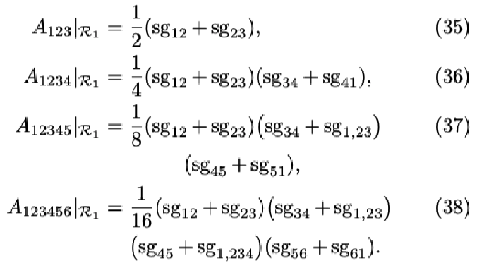
Finally, they conjecture (and then prove) a generalization to arbitrary n:

These results are cool, but that’s not the primary reason why this paper is receiving so much attention. Going back up to the authors list, you’ll see that this work was done in collaboration with OpenAI. Indeed, in a related article ( https://openai.com/index/new-result-theoretical-physics/ ), the team at OpenAI writes,
“A central aspect of the work concerns methodology. The final formula, Eq. (39) in the preprint, was first conjectured by GPT‑5.2 Pro. The human authors worked out the amplitudes for integer n up to n = 6 by hand, obtaining very complicated expressions shown in Eqs. (29)--(32), which correspond to a ‘Feynman diagram expansion’ whose complexity grows superexponentially in n. GPT‑5.2 Pro was able to greatly reduce the complexity of these expressions, providing the much simpler forms in Eqs. (35)--(38). From these base cases, it was then able to spot a pattern and posit a formula valid for all n.”
That is, they credit GPT-5.2 Pro for generating the simplified equations! These were then verified as correct by the researchers.
Several of us at Wolfram saw this paper and became curious: How might we quickly verify the equality of Eqs. 29-32 and Eqs. 35-38 (in) using the Wolfram Language?
This notebook presents the fastest verifications for the n = 3, 4, and 5 cases that we found these last couple of days. Daniele Ceravolo did some numerical investigation, Dennis Foren isolated the underlying mathematical problem from the physics context, and Adam Strzebonski proposed & implemented the method that we use to check equality for n = 4 and 5. While we work on the n = 6 case, we wanted to bring the challenge to Wolfram Community: How would YOU go about demonstrating equality between these sets of equations? We’re confident that y’all can find some creative strategies!
In the next section, we detail the variables and constraints involved in this problem. Afterwards, we go through the n = 3, 4, and 5 cases.
“A central aspect of the work concerns methodology. The final formula, Eq. (39) in the preprint, was first conjectured by GPT‑5.2 Pro. The human authors worked out the amplitudes for integer n up to n = 6 by hand, obtaining very complicated expressions shown in Eqs. (29)--(32), which correspond to a ‘Feynman diagram expansion’ whose complexity grows superexponentially in n. GPT‑5.2 Pro was able to greatly reduce the complexity of these expressions, providing the much simpler forms in Eqs. (35)--(38). From these base cases, it was then able to spot a pattern and posit a formula valid for all n.”
That is, they credit GPT-5.2 Pro for generating the simplified equations! These were then verified as correct by the researchers.
Several of us at Wolfram saw this paper and became curious: How might we quickly verify the equality of Eqs. 29-32 and Eqs. 35-38 (in
R
1
This notebook presents the fastest verifications for the n = 3, 4, and 5 cases that we found these last couple of days. Daniele Ceravolo did some numerical investigation, Dennis Foren isolated the underlying mathematical problem from the physics context, and Adam Strzebonski proposed & implemented the method that we use to check equality for n = 4 and 5. While we work on the n = 6 case, we wanted to bring the challenge to Wolfram Community: How would YOU go about demonstrating equality between these sets of equations? We’re confident that y’all can find some creative strategies!
In the next section, we detail the variables and constraints involved in this problem. Afterwards, we go through the n = 3, 4, and 5 cases.
Definitions
Definitions
Spinors
Spinors
In principle, each gluon has two spinors: and , wherein =(1,) and =(1,), where , , and are independent real numbers. [Eq. 2]These imply the following spinor contractions: = - and = -.Because we’re working in the half-collinear regime, the contractions vanish for all i and j [Eq. 13]. This is equivalent to saying all of the are equal, which makes them irrelevant to the remainder of our investigation. In contrast, we assume all are nonzero, i.e., all ≠ for all i,j ∈ {1, ..., n}.Meanwhile, momentum conservation in the half-collinear regime requires that =0, which implies both =0 and =0. [the in Eq. 16].The region adds another constraint: <0 and > 0 for all j ∈ {2, ..., n}.In our code, we define and below:
λ
i
λ
i
λ
i
z
i
λ
i
ω
i
z
i
ω
i
z
i
z
i
λ
i
λ
j
z
i
z
j
λ
i
λ
j
ω
i
ω
j
z
i
z
j
λ
i
λ
j
z
i
λ
i
λ
j
z
i
z
j
Σ
i
λ
i
Σ
i
w
i
Σ
i
w
i
z
i
2
δ
R
1
ω
1
ω
j
λ
i
λ
i
λ
j
In[]:=
λt[i_]:=ω[i]*{1,zt[i]};λtλt[λti_,λtj_]:=λti[[2]]*λtj[[1]]-λti[[1]]*λtj[[2]];
And the constraint as follows:
R
1
In[]:=
nParticleSpinorWR1[n_]:=Table[If[TrueQ[i==1],ω[i]<0,ω[i]>0],{i,1,n}];nParticleSimplify[n_][X_]:=Simplify[X,nParticleSpinorWR1[n]];
We will primarily use momentum conservation to eliminate and :
ω
1
λ
1
In[]:=
ω1[n_]:=-Sum[ω[i],{i,2,n}];zt1[n_]:=Sum[ω[i]*zt[i],{i,2,n}]/(-ω1[n]);
... and after eliminating the i=1 parameters, we will impose nonzero via:
λ
i
λ
j
In[]:=
nParticleNonzeroλtλt[n_]:=Table[zt[ij[[1]]]!=zt[ij[[2]]],{ij,Select[Tuples[Table[i,{i,2,n}],2],#[[1]]<#[[2]]&]}];
sg
sg
The stripped amplitudes in which we’re interested are written in terms of sign functions, which the authors label as “sg”. There are various definitions of sg throughout the paper, each of which expands the scope of the symbol. Below Eq. 10, the authors write “sg(x) = 2Θ(x) - 1 denotes the sign function and Θ(x) is the step function.” This is extended first in Eq. 10 and then further above Eq. 29. We summarize these rules like so:
In[]:=
sg[x_]:=RealSign[x];sg[i_,j_]:=RealSign[λtλt[Sum[λt[ix],{ix,i}],Sum[λt[jx],{jx,j}]]];
Equations
Equations
Finally, here are the equations we’re interested in:
(*Eqs.35-38*)Eq["simple",3]=1/2*(sg[{1},{2}]+sg[{2},{3}]);Eq["simple",4]=1/4*(sg[{1},{2}]+sg[{2},{3}])*(sg[{3},{4}]+sg[{4},{1}]);Eq["simple",5]=1/8*(sg[{1},{2}]+sg[{2},{3}])*(sg[{3},{4}]+sg[{1},{2,3}])*(sg[{4},{5}]+sg[{5},{1}]);Eq["simple",6]=1/16*(sg[{1},{2}]+sg[{2},{3}])*(sg[{3},{4}]+sg[{1},{2,3}])*(sg[{4},{5}]+sg[{1},{2,3,4}])*(sg[{5},{6}]+sg[{6},{1}]);
(*Eq.39*)Eq["general",3]=1/2*(sg[{2},{3}]+sg[{1},{2}]);Eq["general",4]=Eq["general",3]*1/2*(sg[{3},{4}]+sg[{1},{2,3}]);Eq["general",5]=Eq["general",4]*1/2*(sg[{4},{5}]+sg[{1},{2,3,4}]);Eq["general",6]=Eq["general",5]*1/2*(sg[{5},{6}]+sg[{1},{2,3,4,5}]);
n = 3
n = 3
Let’s start with the n = 3 case, wherein we wish to show Eq. 29 and Eq. 35 are equivalent. These are, respectively,
In[]:=
n=3;Eq29=Eq["complex",3]Eq35=Eq["simple",3]
Out[]=
RealSign[zt[1]ω[1]ω[2]-zt[2]ω[1]ω[2]]
Out[]=
1
2
First, let’s eliminate and from the equations:
ω
1
z
1
In[]:=
outANo1=Eq29/.{ω[1]->ω1[n],zt[1]->zt1[n]}outBNo1=Eq35/.{ω[1]->ω1[n],zt[1]->zt1[n]}
Out[]=
RealSign-zt[2]ω[2](-ω[2]-ω[3])+
ω[2](-ω[2]-ω[3])(zt[2]ω[2]+zt[3]ω[3])
ω[2]+ω[3]
Out[]=
1
2
ω[2](-ω[2]-ω[3])(zt[2]ω[2]+zt[3]ω[3])
ω[2]+ω[3]
These can then be simplified via the n-particle constraints:
In[]:=
outA=nParticleSimplify[n][outANo1]outB=nParticleSimplify[n][outBNo1]
Out[]=
RealSign[zt[2]-zt[3]]
Out[]=
RealSign[zt[2]-zt[3]]
which reveals they’re equivalent! i.e., their difference is zero:
In[]:=
diff=outA-outB
Out[]=
0
Thus, Eqs. 29 and 35 are equivalent in .
R
1
n = 4
n = 4
Next, we attempt to show that the n = 4 amplitudes Eq. 30 and Eq. 36 are equivalent. These are, respectively,
In[]:=
n=4;Eq30=Eq["complex",n]Eq36=Eq["simple",n]
Out[]=
1
2
Out[]=
1
4
We once again remove the i=1 parameters from each and take their difference:
In[]:=
outANo1=Eq30/.{ω[1]->ω1[n],zt[1]->zt1[n]}outBNo1=Eq36/.{ω[1]->ω1[n],zt[1]->zt1[n]}
Out[]=
1
2
ω[2](-ω[2]-ω[3]-ω[4])(zt[2]ω[2]+zt[3]ω[3]+zt[4]ω[4])
ω[2]+ω[3]+ω[4]
(-ω[2]-ω[3]-ω[4])ω[4](zt[2]ω[2]+zt[3]ω[3]+zt[4]ω[4])
ω[2]+ω[3]+ω[4]
Next, let’s find all of the combinations of RealSign values that would yield a nonzero value for the amplitude difference:
Recall that our parameter space is constrained via...
n = 5
n = 5
We approach the n = 5 case just as we did the n = 4 case:
While the previous implementation works fine in this case, we can further speed things up via parallelization:
CITE THIS NOTEBOOK
CITE THIS NOTEBOOK
Investigating equality of stripped gluon amplitudes
by Dennis Foren
Wolfram Community, STAFF PICKS, February 20, 2026
https://community.wolfram.com/groups/-/m/t/3642590
by Dennis Foren
Wolfram Community, STAFF PICKS, February 20, 2026
https://community.wolfram.com/groups/-/m/t/3642590