ABSTRACT (original article): A single equation of state (EOS) such as the Peng-Robinson (PR) EOS can accurately describe both the liquid and vapor phase. We present several applications of this equation of state, including estimation of pure component properties and computation of the vapor-liquid equilibrium (VLE) diagram for binary mixtures. We perform high-pressure chemical-equilibrium calculations. Finally, we solve an adiabatic flash distillation problem for a multi- component mixture. All these computations are available in electronic format in the form of MATLAB® programs upon request from the authors or from the File Exchange Center. These problems can serve as teaching material for a chemical engineering thermodynamics undergraduate level course. CITATION (original article): Nasri Z. & Binous H. (2009). Applications of the peng-robinson equation of state using Matlab. Chemical Engineering Education Vol. 43 No. 2 115–124. https://journals.flvc.org/cee/article/view/122327
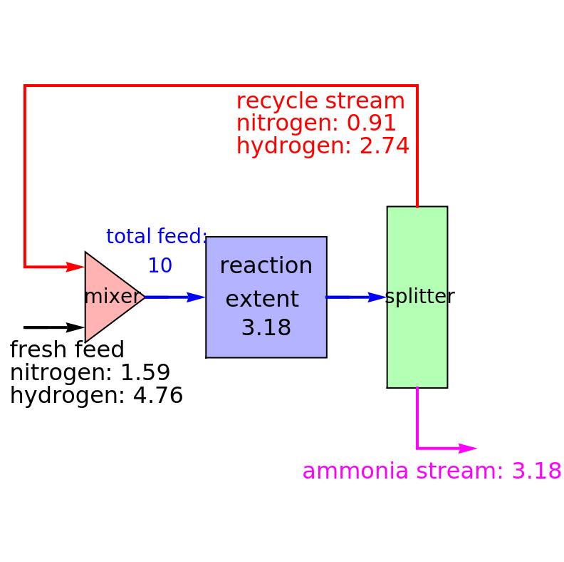
Consider the high-pressure synthesis of ammonia (), known as the Haber process.
1.5+0.5⇋
H
2
N
2
NH
3
We use the Peng–Robinson equation of state and the reaction-coordinate method to compute the extent of reaction, in moles of per unit time (e.g., hours), for the reactor temperature (in degrees Kelvin) and pressure (in bars): 600 K and 100 bar.
ξ
NH
3
T
P
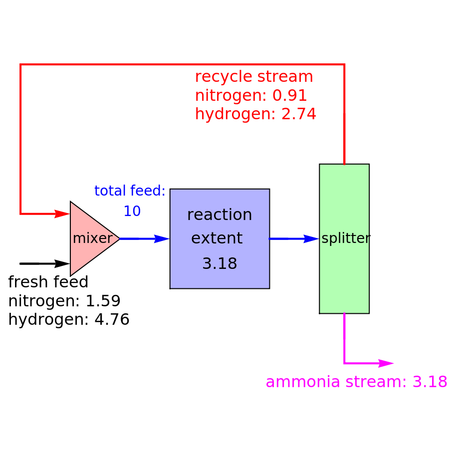
We carry out the mass balance around the reactor and splitter in order to compute the amount of ammonia produced when chemical equilibrium is reached in the reactor and in the recycle stream. To do so, we assume that: (1) the splitter separates the product (i.e., ammonia) perfectly from the reactants (i.e., nitrogen and hydrogen); and (2) the fresh feed contains stoichiometric amounts of nitrogen and hydrogen.
As expected from Le Chatelier’s principle, if you try other values of T and P, the amount of ammonia produced will be greater at low temperatures and high pressures.
reactor’s conditions and inlet feed flow rate
In[]:=
T=600;(*temperature*)P=100;(*pressure*)
In[]:=
feed=10;(*reactorfeedflowrate*)
Peng–Robinson equation of state
In[]:=
R=8.314;(*universalgasconstant*)
In[]:=
(*interactionparametersfromAspen-Hysys*)k[1,1]=0;k[2,2]=0;k[3,3]=0;k[2,1]=k[1,2];k[3,1]=k[1,3];k[2,3]=k[3,2];k[1,2]=-0.036;k[1,3]=0;k[3,2]=0.222;
Tre[i_]:=T/Tc[i];(*reducedtemperature*)ap[i_]:=0.45724a[i]R^2Tc[i]^2/Pc[i];Ap[i_,P_]:=ap[i]P/(RT)^2;bp[i_]:=0.07780RTc[i]/Pc[i];Bp[i_,P_]:=Pbp[i]/(RT);(*gas-phasefugacitycoefficients*)ϕv[i_,P_]:=Exp(Zv-1)Bp[i,P]Bv[P]-Log[Zv-Bv[P]]-Av[P]2y[j]Ab[i,j,P]Av[P]-Bp[i,P]Bv[P]LogZv+1+y[i]y[j]Ab[i,j,P];Ab[i_,j_,P_]:=(Ap[i,P]Ap[j,P])^0.5(1-k[i,j]);Bv[P_]:=y[i]Bp[i,P];
2
Bv[P]23
∑
j=1
2
Bv[P]Zv+1-2
Bv[P];a[i_]:=(1+m[i](1-Tre[i]^0.5))^2;m[i_]:=0.37464+1.54226ω[i]-0.26992ω[i]^2;Av[P_]:=3
∑
i=1
3
∑
j=1
3
∑
i=1
(*criticalpressureandtemperatureandaccentricfactor*)Pc[1]=13.0;Tc[1]=33.2;ω[1]=-0.22;(*hydrogen*)Pc[2]=33.9;Tc[2]=126.2;ω[2]=0.04;(*nitrogen*)Pc[3]=112.8;Tc[3]=405.6;ω[3]=0.25;(*ammonia*)
The reaction-coordinate method is used to compute the extent of reaction, ξ
y[1]=1-y[2]-y[3];(*summationrule*)y[3]=;y[2]=;(*materialbalanceequations*)Ka298=Exp[16.51000/(R298.15)];(*equilibriumconstantat25°C*)ΔH[T_]:=-46100+(T-298.15)Δa+Δb/2(T^2-298.15^2)+Δc/3(T^3-298.15^3)+Δd/4(T^4-298.15^4);Δa=24.619-0.5×27.318-1.5×26.879;Δb=(3.75-0.5(0.623)-1.5(0.435))10^-2;Δc=(-0.138+0.5(0.095)+1.5(0.033))10^-5;Δd=(0.5(2.871)+1.5(0.87))10^-9;Ka[T_]:=Ka298Exp[Δa/8.314Log[T/298.15]+Δb/(2×8.314)(T-298.15)+Δc/(6×8.314)(T^2-298.15^2)+Δd/(12×8.314)(T^3-298.15^3)+1/8.314(46100+(298.15)Δa+Δb/2(298.15^2)+Δc/3(298.15^3)+Δd/4(298.15^4))(1/T-1/298.15)];(*equilibriumconstantatT*)
ξ
feed-ξ
feed/4-0.5ξ
feed-ξ
In[]:=
(*solvingforthecompressibilityfactor(Z)andtheextentofreaction(ξ)*)sol=Quiet@FindRoot[{Ka[T]*(y[2])^0.5(y[1])^1.5(ϕv[1,P]^1.5ϕv[2,P]^0.5)y[3]/(P/1.0)ϕv[3,P],Zv^3+(-1+Bv[P])Zv^2+Zv(Av[P]-3Bv[P]^2-2Bv[P])-Av[P]Bv[P]+Bv[P]^2+Bv[P]^30},{Zv,0.9},{ξ,0.5}]
Out[]=
{Zv0.998473,ξ3.17565}
In[]:=
(*recyclestreamcomposition*)sol1=Solve[(feed/4.-(ξ/.sol)/2)recycledN,recycledN]sol2=Solve[(feed3./4.-(ξ/.sol)/23)recycledH,recycledH]
Out[]=
{{recycledN0.912175}}
Out[]=
{{recycledH2.73653}}
In[]:=
(*drawingthecalculatedflowsheet*)Show[Graphics[{EdgeForm[Black],Blue,Opacity[0.3],Rectangle[{-2,-2},{2,2}],Red,Polygon[{{-6,-1.5},{-4,0},{-6,1.5}}],Opacity[1],Thick,Black,Arrow[{{-8,-1},{-6,-1}}],Blue,Arrow[{{-4,0},{-2,0}}],Blue,Arrow[{{2,0},{4,0}}],Green,Opacity[0.3],Rectangle[{4,-3},{6,3}],Thick,Black,Opacity[1],Magenta,Arrow[{{5,-3},{5,-5},{7,-5}}],Red,Arrow[{{5,3},{5,7},{-8,7},{-8,1},{-6,1}}],Style[Text[" splitter",{5,0},{0,0}],Black,14],,Style[Text["mixer",{-5.1,0},{0,0}],Black,14],Style[Text[Row[{"reaction","\n","extent "}],{0,0.5},{0,0}],Black,16],Style[Text[NumberForm[ξ/.sol,{3,2}],{0,-1},{0,0}],Black,16],Style[Text["recycle stream",{-1,6.5},{-1,0}],Red,16],Style[Text[Row[{"nitrogen: ",NumberForm[recycledN/.sol1//First,{3,2}]}],{-1,5.75},{-1,0}],Red,16],Style[Text[Row[{"hydrogen: ",NumberForm[recycledH/.sol2//First,{3,2}]}],{-1,5.0},{-1,0}],Red,16],Style[Text["fresh feed",{-8.5,-1.75},{-1,0}],Black,16],Style[Text[Row[{"nitrogen: ",NumberForm[First[feed/4.-recycledN/.sol1],{3,2}]}],{-8.5,-2.5},{-1,0}],Black,16],Style[Text[Row[{"hydrogen: ",NumberForm[First[feed3/4.-recycledH/.sol2],{3,2}]}],{-8.5,-3.25},{-1,0}],Black,16],Style[Text[Row[{"ammonia stream: ",NumberForm[(ξ/.sol),{3,2}]}],{5.5,-5.75},{0,0}],Magenta,16],Style[Text[Row[{"total feed: ","\n",NumberForm[feed,{3,2}]}],{-3.5,1.5},{0,0}],Blue,14]}],ImageSize{450,450}]
Out[]=
CITE THIS NOTEBOOK
CITE THIS NOTEBOOK
Mass balance in the Haber process
by Housam Binous and Ahmed Bellagi
Wolfram Community, STAFF PICKS, March 17, 2024
https://community.wolfram.com/groups/-/m/t/3113178
by Housam Binous and Ahmed Bellagi
Wolfram Community, STAFF PICKS, March 17, 2024
https://community.wolfram.com/groups/-/m/t/3113178