Problem
Problem
Out[]=
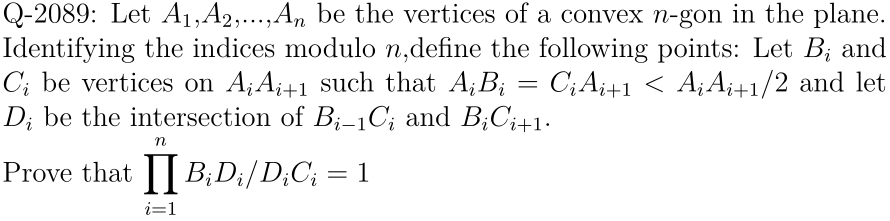
Tips for visualization
Tips for visualization
Generate “usable” convex polygons
Generate “usable” convex polygons
You can use RandomPolygon[{“Convex”,n}] to generate any convex n-gon in general, but in (uncountably) many cases it is bad configuration for our solution. For example:
Graphics[{Transparent,EdgeForm[Thick],BlockRandom[RandomPolygon[{"Convex",5}],RandomSeeding667]}]
Out[]=
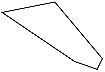
Comparing to the polygon I used in the animation, the figure above has a really short side and a almost-flat obtuse angle. It is impossible to put point B’s and C’s on this side without covering vertices and one triangle is going to be flat. So the ideal case should have
B
i
D
i
C
i
◼
relatively even side lengths
◼
enough space in the polygon
The translation in mathematical words of these requirements is choosing a random polygon some what close to a regular polygon, which has even side lengths and maximum area given a fixed circumference. Here is a quite handy heuristic implementation:
use CirclePoints to generate vertices for a regular polygon and slightly perturb them so that we break the convex property.
use CirclePoints to generate vertices for a regular polygon and slightly perturb them so that we break the convex property.
In[]:=
n=5;
poly=(RandomReal[{-0.3,0.3},2]+#)&/@CirclePoints[2,n];Graphics[{Transparent,EdgeForm[Thick],Polygon@poly}]
Out[]=
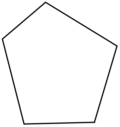
Then we can assign A’s to the generated coordinates of the polygon above. Note that I use Mod[m,n,1] for new indices because we need index goes back to 1
n+1
In[]:=
ptA[id_,n_]:=poly[[Mod[id,n,1]]]
Add B’s and C’s onto the edges of polygon A1A2A3...An-1An
Add B’s and C’s onto the edges of polygon ...
A
1
A
2
A
3
A
n-1
A
n
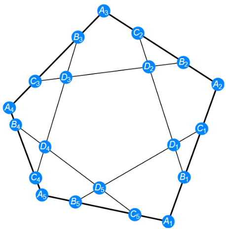
For example we have a pentagon and and we can find the coordinates of B’s using simple affine transformation: (-)+ . Using the fact that , the coordinate of C’s are (1-)(-)+ :
λ,,,,{,,,,}
A
1
B
1
A
1
A
2
A
2
B
2
A
2
A
3
A
3
B
3
A
3
A
4
A
4
B
4
A
4
A
5
A
5
B
5
A
5
A
1
λ
1
λ
2
λ
3
λ
4
λ
5
B
i
λ
i
A
i+1
A
i
A
i
A
i
B
i
C
i
A
i+1
C
i
λ
i
A
i+1
A
i
A
i
In[]:=
λ=RandomReal[{0.17,0.38},n];
In[]:=
ptB[id_,n_]:=λ[[Mod[id,n,1]]]*(ptA[id+1,n]-ptA[id,n])+ptA[id,n]
In[]:=
ptC[id_,n_]:=(1-λ[[Mod[id,n,1]]])*(ptA[id+1,n]-ptA[id,n])+ptA[id,n]
The bound from 0.17 to 0.38 is set so B’s and C’s are far away from A’s and each other. This is a fairly good choice for clear visualization and satisfying the condition in the problems at the same time.
Solve D’s
Solve D’s
The coordinates are directly from the instruction from the problem
In[]:=
ptD=LineLineIntersection[Table[{ptB[k,n],ptC[k+1,n],ptC[k,n],ptB[k-1,n]},{k,1,n}]];
Verify the conclusion
Verify the conclusion
Product of the length of for from to
B
i
C
i
i
1
n
Times@@MapThread[EuclideanDistance,{Table[ptB[k,n],{k,n}],ptD}]
Out[]=
0.0424957
Product of the length of for from to
C
i
D
i
i
1
n
Times@@MapThread[EuclideanDistance,{Table[ptC[k,n],{k,n}],ptD}]
Out[]=
0.0424957
Animation
Animation
Wrap up everything above into a Dynamic expression. Changing n to see how this code handles arbitrary polygon while the Dynamic expression is updating :
In[]:=
n=6;
Dynamic[Refresh[λ=RandomReal[{0.17,0.38},n];poly=(RandomReal[{-0.3,0.3},2]+#)&/@CirclePoints[2,n];ptD=LineLineIntersection[Table[{ptB[k,n],ptC[k+1,n],ptC[k,n],ptB[k-1,n]},{k,1,n}]];Graphics[{{Transparent,EdgeForm[Thick],Polygon[poly]},Line[Table[{ptB[k,n],ptC[k+1,n]},{k,n}]],MapThread[label[#1,ptA[#2,n]]&,{Table[StringForm["",k],{k,n}],Range[n]}],MapThread[label[#1,ptB[#2,n]]&,{Table[StringForm["",k],{k,n}],Range[n]}],MapThread[label[#1,ptC[#2,n]]&,{Table[StringForm["",k],{k,n}],Range[n]}],MapThread[label[#1,ptD[[#2]]]&,{Table[StringForm["",k],{k,n}],Range[n]}]},PlotRange->2.2*{{-1,1},{-1,1}}],UpdateInterval1]]
A
`1`
B
`1`
C
`1`
D
`1`
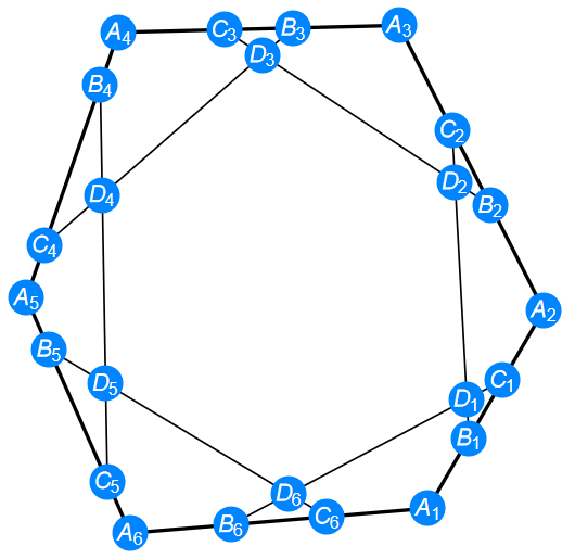
Sketch of the proof
Sketch of the proof
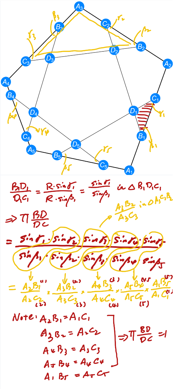
Nieto posted an elegant solution with little words. See my illustration using pentagon as example. Basically we convert between side ratios and trigonometric ratio (using the law of sines) in small shaded triangle ( like ) and large triangle (like ) alternatively. Using and we find that in the last step the numerator is just a permutation of the denominator, then we can conclude the statement in the problem is true.
B
k
C
k
D
k
A
k
B
k-1
C
k
A
k
B
k
C
k
A
k+1
Utility function
Utility function