Arc-Length Continuation of Common Tangent Plane Solutions in UNIQUAC-Based Liquid-Liquid Equilibrium
Authors: Housam Binous
Arc-Length Continuation of Common Tangent Plane Solutions in UNIQUAC-Based Liquid-Liquid Equilibrium
Authors: Housam Binous
Authors: Housam Binous
The liquid–liquid equilibrium (LLE) behavior of the ternary system consisting of isobutyl acetate, acetic acid, and water at 283.15 K was modeled using the UNIQUAC activity coefficient model. The binary interaction parameters and the UNIQUAC parameters (i.e., r and q) reported by Cháfer et al. were used to calculate activity coefficients and the excess Gibbs free energy of mixing. The dimensionless Gibbs energy surface, (g/RT), was formulated as a function of composition and served as the thermodynamic basis for determining phase stability and phase splitting. The UNIQUAC model captures the strong non-ideal interactions present in partially miscible liquid systems and is therefore well suited for describing liquid–liquid equilibria in this ternary mixture.
The equilibrium compositions of the two coexisting liquid phases were determined using the common tangent plane criterion. This approach requires that the Gibbs free energy surface possess a common tangent plane touching the surface at two distinct compositions corresponding to the equilibrium phases. Mathematically, the method involves solving a set of nonlinear equations that enforce equality of the tangent plane slopes and satisfy the Gibbs energy balance between the two phase compositions. An additional distance constraint was introduced to prevent convergence toward the trivial solution where both phases have identical compositions. The resulting system of equations defines a point on the binodal curve and provides the basis for tracing the complete liquid–liquid equilibrium boundary.
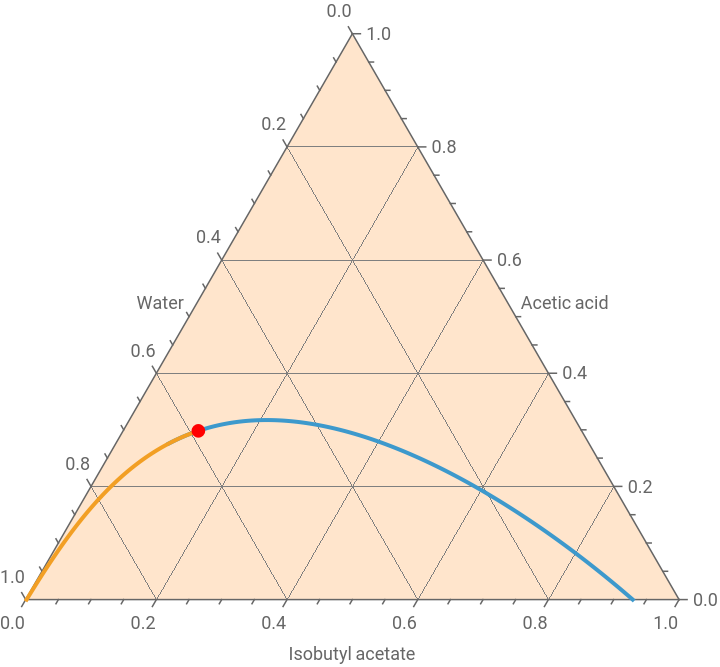
To generate the entire coexistence curve, a continuation technique based on arc-length parameterization was employed. Starting from an initial equilibrium solution obtained by FindRoot, the common tangent plane equations were transformed into a differential-algebraic system and solved using NDSolve. The continuation variable enabled smooth progression along the equilibrium manifold, allowing the binodal curve to be traced from one end of the two-phase region to the other. The method simultaneously produced the compositions of both equilibrium phases and identified the plait point, corresponding to the critical composition where the two liquid phases become indistinguishable.
The last Figure presents the calculated ternary phase diagram together with experimental data reported by Cháfer et al. The blue and yellow curve represents the predicted binodal boundary separating the single-phase and two-phase regions, while the red point indicates the calculated plait point. Red tie-lines connect the compositions of the two coexisting phases predicted by the UNIQUAC model, whereas the blue dashed tie-lines correspond to experimental measurements reported in Ref. 1. The overall agreement between calculated and experimental results demonstrates the ability of the UNIQUAC model combined with the common tangent plane continuation method to accurately reproduce the liquid–liquid equilibrium behavior of the isobutyl acetate–acetic acid–water system. Small deviations observed near the plait point are expected due to the increased sensitivity of phase compositions in the critical region.
Reference:
[1] A. Cháfer, E. Lladosa, J. de la Torre, M.C. Burguet, Study of liquid–liquid equilibrium of the systems isobutyl acetate+acetic acid+water and isobutyl alcohol+acetic acid+water at different temperatures, Fluid Phase Equilibria, Volume 271, Issues 1–2, 2008, Pages 76-81, https://doi.org/10.1016/j.fluid.2008.07.001
Method based on common tangent plane and arc-length continuation
In[]:=
ClearAll["Global`*"];
(*UNIQUACModel-Cháferetal.,FluidPhaseEquilibria271(2008)*)(*ParametersatT=283.15K,Table4*)R=8.314;(*J/(molK)*)T=283.15;(*K*)(*System:Isobutylacetate(1)+Aceticacid(2)+Water(3)*)r={4.8266,2.2023,0.9200};q={4.1918,2.072,1.3997};(*----------InteractionparametersAij(J/mol),Table4@283.15K----------*)(*System1:Isobutylacetate(1)+Aceticacid(2)+Water(3)*)Auniquac={{0,-1022.71,4023.77},{154.58,0,-1622.51},{965.14,762.46,0}}/R/T;
In[]:=
Auniquac//MatrixForm
Out[]//MatrixForm=
0. | -0.434436 | 1.70925 |
0.0656639 | 0. | -0.689225 |
0.409981 | 0.323885 | 0. |
In[]:=
(*UNIQUACACTIVITYCOEFFICIENTFUNCTION*)lnGamma[x1_,x2_]:=Module[{nc,phi,theta,tau,lnGammaComb,lnGammaRes,lnGamma,z0=10,l,S,sumXL,x},x={x1,x2,1-x1-x2};nc=Length@x;(*Coordinationnumberz0=10*)l=Table[(z0/2)(r[[i]]-q[[i]])-(r[[i]]-1),{i,1,nc}];(*Segment&surfacefractions*)phi=(r*x)/(r.x);theta=(q*x)/(q.x);(*UNIQUACtaumatrix*)tau=Table[Exp[-Auniquac[[i,j]]],{i,1,nc},{j,1,nc}];(*---Combinatorialpart---*)sumXL=Sum[x[[i]]l[[i]],{i,1,nc}];lnGammaComb=Table[Log[phi[[i]]/x[[i]]]+(z0/2)q[[i]]Log[theta[[i]]/phi[[i]]]+l[[i]]-(phi[[i]]/x[[i]])sumXL,{i,1,nc}];(*---Residualpart---*)S=Table[Sum[theta[[j]]tau[[j,i]],{j,1,nc}],{i,1,nc}];lnGammaRes=Table[q[[i]](1-Log[S[[i]]]-Sum[theta[[k]]tau[[i,k]]/S[[k]],{k,1,nc}]),{i,1,nc}];lnGamma=lnGammaComb+lnGammaRes;lnGamma];
In[]:=
(*COMPOSITIONVECTOR*)xvec[x1_,x2_]:={x1,x2,1-x1-x2};gamma[i_,x1_,x2_]:=Exp[lnGamma[x1,x2][[i]]];(*DIMENSIONLESSGIBBSENERGYOFMIXING:g/RT*)gmix[x1_,x2_]:=Module[{x},x=xvec[x1,x2];Sum[x[[i]]Log[x[[i]]],{i,1,3}]+Sum[x[[i]]lnGamma[x1,x2][[i]],{i,1,3}]];(*DERIVATIVES*)dgdx1[x1_,x2_]:=Evaluate[D[gmix[u,v],u]/.{u->x1,v->x2}];dgdx2[x1_,x2_]:=Evaluate[D[gmix[u,v],v]/.{u->x1,v->x2}];(*UNKNOWNS*)vars={x1a,x2a,x1b,x2b,m1,m2};(*COMMONTANGENTEQUATIONS*)eq1=dgdx1[x1a,x2a]==m1;eq2=dgdx1[x1b,x2b]==m1;eq3=dgdx2[x1a,x2a]==m2;eq4=dgdx2[x1b,x2b]==m2;eq5=gmix[x1b,x2b]-gmix[x1a,x2a]==m1(x1b-x1a)+m2(x2b-x2a);(*EXTRACONSTRAINT-Preventtrivialsolutionxα=xβ*)eq6=(x1b-x1a)^2+(x2b-x2a)^2==d;
In[]:=
(*firstvalueford---verysmalld=0.001yieldapproximatelytheplaitpoint*)d0t=0.001;
In[]:=
(*solution*)solct=FindRoot[{eq1,eq2,eq3,eq4,eq5,eq6/.d->d0t},{{x1a,0.5},{x2a,0.25},{x1b,0.6},{x2b,0.26},{m1,-10.0},{m2,40}},MaxIterations->10000]
Out[]=
{x1a0.0811611,x2a0.275855,x1b0.10707,x2b0.293986,m1-0.687507,m2-1.6404}
In[]:=
init={x1a[0]==(x1a/.solct),x2a[0]==(x2a/.solct),x1b[0]==(x1b/.solct),x2b[0]==(x2b/.solct),m1[0]==(m1/.solct),m2[0]==(m2/.solct),d[0]==d0t}
Out[]=
{x1a[0]0.0811611,x2a[0]0.275855,x1b[0]0.10707,x2b[0]0.293986,m1[0]-0.687507,m2[0]-1.6404,d[0]0.001}
In[]:=
initdev={x1a'[0]==-0.0001,x2a'[0]==0.0001,x1b'[0]==0.0001,x2b'[0]==0.0001,m1'[0]==0.01,m2'[0]==0.01,d'[0]==0.00001}
Out[]=
{[0]-0.0001,[0]0.0001,[0]0.0001,[0]0.0001,[0]0.01,[0]0.01,[0]0.00001}
′
x1a
′
x2a
′
x1b
′
x2b
′
m1
′
m2
′
d
In[]:=
SYS={eq1,eq2,eq3,eq4,eq5,eq6}/.x1a->x1a[s]/.x1b->x1b[s]/.x2a->x2a[s]/.x2b->x2b[s]/.m1->m1[s]/.m2->m2[s]/.d->d[s];
In[]:=
auxeq=x1a'[s]^2+x1b'[s]^2+x2a'[s]^2+x2b'[s]^2+m1'[s]^2+m2'[s]^2+d'[s]^2==1
Out[]=
2
′
d
2
′
m1
2
′
m2
2
′
x1a
2
′
x1b
2
′
x2a
2
′
x2b
In[]:=
SYSFinal=Join[SYS,{auxeq},init,initdev];
In[]:=
SOL=Quiet@NDSolve[SYSFinal,{x1a,x2a,x1b,x2b,m1,m2,d},{s,-10,100},AccuracyGoal->5];
In[]:=
DATA1=Table[{x1a[s],x2a[s],1-x1a[s]-x2a[s]}/.SOL,{s,0,12.355,0.001}];DATA2=Table[{x1b[s],x2b[s],1-x1b[s]-x2b[s]}/.SOL,{s,0,12.355,0.001}];
In[]:=
Pt={{2,1},{0,Sqrt[3.]}}/2;
Type I liquid-liquid equilibrium (LLE) diagram - Plait point indicated in red
In[]:=
p0=Show[TernaryListPlot[{Flatten[DATA1,1],Flatten[DATA2,1]},Joined->True,PlotStyle->Thick,GridLines->Automatic,FrameLabel->{"Isobutyl acetate","Acetic acid","Water"},PlotRange->All,Method->{"Backdrop"->LightOrange}],Graphics[{Red,PointSize[0.02],Point[Pt.{x1a[s],x2a[s]}/.SOL/.s->0.06]}]]
Out[]=
In[]:=
(*data*)(*ExperimentalLLEdata-Table2*)(*Isobutylacetate(1)+Aceticacid(2)+Water(3)*)(*T=283.15K*)(*Columns:x1,x2foreachphase(x3=1-x1-x2)*)(*Isobutylacetate-richphase:{x1,x2}*)acetateRichPhase283={{0.945,0.000},{0.892,0.020},{0.847,0.054},{0.792,0.092},{0.744,0.120},{0.704,0.140},{0.664,0.159},{0.615,0.187},{0.572,0.206},{0.522,0.227},{0.483,0.248},{0.447,0.264},{0.412,0.275},{0.363,0.289},{0.320,0.295},{0.265,0.309},{0.205,0.314}};(*Water-richphase:{x1,x2}*)waterRichPhase283={{0.001,0.000},{0.002,0.011},{0.001,0.023},{0.002,0.038},{0.002,0.049},{0.002,0.057},{0.003,0.068},{0.003,0.079},{0.004,0.089},{0.005,0.100},{0.005,0.116},{0.006,0.128},{0.008,0.139},{0.011,0.158},{0.015,0.173},{0.024,0.199},{0.040,0.227}};(*Addx3column(water/acetate,bydifference)andfulltriples*)acetateRichFull283=Map[Append[#,1-Total[#]]&,acetateRichPhase283];waterRichFull283=Map[Append[#,1-Total[#]]&,waterRichPhase283];(*Displayastableswithheaders*)TableForm[acetateRichFull283,TableHeadings->{None,{"x1 (acetate)","x2 (acetic acid)","x3 (water)"}}]TableForm[waterRichFull283,TableHeadings->{None,{"x1 (acetate)","x2 (acetic acid)","x3 (water)"}}]