I analyzed the amount of supermarkets in low-access areas with varying radii. This was done through a series of functions that used a tandem of coordinates and geographical Entities (cities, U.S counties, etc.). The overall goal of this project was to highlight disadvantaged communities’ needs for accessibility to nutrition, and to underscore the importance of attending to the right to food access. My research led me to find that while the United States is known to be a place of opportunity and prosperity, certain areas are plagued by low access to proper nutrition. These areas primarily include counties from states in the west such as Arizona, New Mexico, and Nevada.
Introduction
Introduction
Food deserts are defined the by the United States Department of Agriculture (USDA) as an area with limited access to supermarkets, super-centers, grocery stores, or any other source of healthy and affordable food. This definition can have two different meanings: First, a certain proportion of the U.S. population doesn’t have access to basic nutritional necessity, and second, even if food is accessible, it does not contribute to a healthy diet. In fact, it is estimated that more than 23 million people live in low-income or rural neighborhoods that are more than a mile away from a supermarket. During my research for school and extracurricular activities, I stumbled upon the limits of the country’s welfare programs and their capabilities. I decided to further explore these issues in a computational manner primarily with the GeoData functions.
Overview of the Food Access Research Atlas
Overview of the Food Access Research Atlas
The primary data resource utilized in this research project was the Food Access Research Atlas, composed and analyzed by the USDA.
In[]:=
fara=ResourceObject["Food Access Research Atlas"]
Out[]=
ResourceObject


The Food Access Research Atlas allows users to access data in regards to food access across the United States. For those who utilize the dataset to extract certain points of data from specific parameters, the Research Atlas provides a plethora of variables to explore.
In[]:=
Keys[fara][[1]]
Out[]=
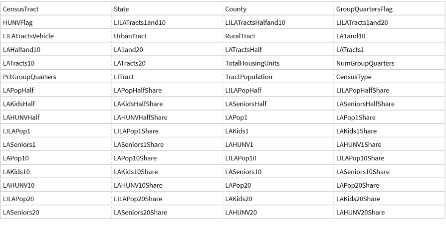
These variables range from “LATracts10”, which represents data regarding “Low-Access Tracts to Food, 10 miles” , to more specific parameters, such as LILAPop20, “Low Income and Low Access Population, 20 miles”.
FARA Visualization
FARA Visualization
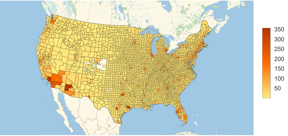
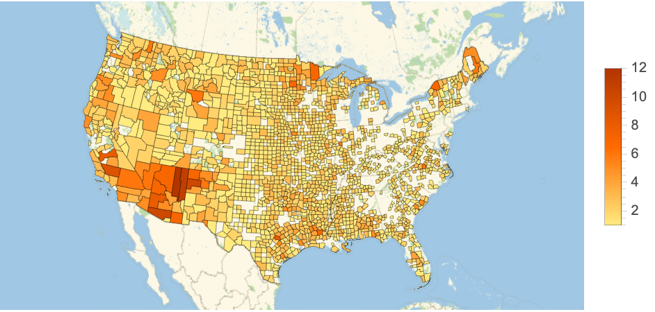
Using the “LATracts1”, “LATracts10”, and “LATracts20” parameters that are part of the FARA’s variables, counties with low access to affordable, nutritious food at stages of 1, 10, and 20 mile radii are represented.
Using the LATracts1 variable, we get all the areas with low access to nutritional retailers within 1 mile:
In[]:=
latracts1[]:=GeoRegionValuePlotLength/@GroupBy[ResourceData["Food Access Research Atlas"][Select[#LATracts1==True&]],"County"],GeoRange->
In[]:=
latracts1[]
Out[]=
Areas with low access to nutritional retailers within 10 miles :
latracts10[]:=GeoRegionValuePlotLength/@GroupBy[ResourceData["Food Access Research Atlas"][Select[#LATracts10==True&]],"County"],GeoRange->
latracts10[]
Out[]=
Areas with low access to nutritional retailers within 20 miles :
latracts20[]:=GeoRegionValuePlotLength/@GroupBy[ResourceData["Food Access Research Atlas"][Select[#LATracts20==True&]],"County"],GeoRange->
latracts20[]
Out[]=
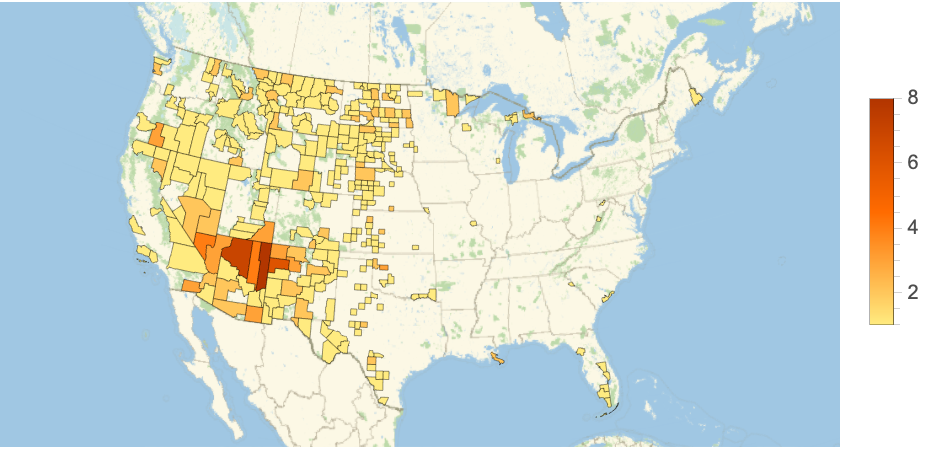
In each of these cases, the GeoRegionValuePlot[] function is used to color in areas that have multiple cities that do not have accessible food retailers at one, ten, or twenty miles. This is performed by extracting the specific “LATracts” column in the FALA. The data type of this column is a boolean (True/False) because a region can either have access to food within a certain amount of miles, or it cannot. In each county, the amount of True values are tallied into a list, and the length of the list is extracted. The heat bar on the right of the map provides insight as to how many cities in each county are affected by the given condition, which is also the length of the list.
Overview of SNAP Programs
Overview of SNAP Programs
The Supplemental Nutrition Assistance Program, better known as “SNAP” is a federal program aimed at providing funds to low-income families to use for healthy food. This helps recipients allocate their money elsewhere and move towards self-sufficiency by using SNAP credits on nutrition. The Casey Foundation Data Center found that nearly 41.5 million people receive SNAP benefits. However, not all retailers are allowed to accept SNAP benefits as a means of payment, and must be authorized. Thus, access is crucial to optimize retailer locations, as these benefits mean nothing without close proximity to one of the approved SNAP retailers.
SNAP Retailer Dataset Components
SNAP Retailer Dataset Components
As such, this SNAP Retailer dataset, provided by the USDA, gives insight into specified locations of SNAP-approved retailers .
A table of all the contents of the SNAP Retailers data :
In[]:=
SNAPData=ResourceData["SNAP Retailers"]
Out[]=
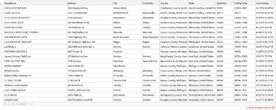
Primarily, the data variables used to locate and analyze these SNAP retailers were “StoreName”, “City”, “CityEntity”, “State”, and “Coordinates”.
Applying the SNAP Dataset
Applying the SNAP Dataset
Using the “Coordinates” column of the dataset, the user can input latitude, longitude, and a specified radius to determine the closest SNAP retailers within that area.
A function that determines the most accessible retailers closest to the inputted distance:
In[]:=
listInput[lat_,lon_,rad_]:=Table[If[GeoDistance[SNAPData[[i,"Coordinates"]],{lat,lon}]<=rad,SNAPData[[i]],Nothing],{i,100000}]
In[]:=
listInput[40.7128,-74.0060,Quantity[5,"Miles"]]
Out[]=
,
,
Using the GeoDistance[] function, longitude and latitude variables are able to be processed so that coordinates from the dataset can be used to form a distance between the points. Additionally, because the dataset contains upwards of 250,000 locations, the first 100,000 locations were processed, which can be changed.
With the same logic, we are able to plot points of the stores above in relation to the given longitude and latitude:
Here, the use of a module allows us to store the initial function (listInput) in an accessible variable. From here, the GeoListPlot[] function does the work for us, marking the stores with red points. To achieve this result, we use the “Coordinates” column to find the precise location.
Rather than only analyzing user-inputted coordinates, taking in cities as entities allows for a simpler interface.
A function that points out all SNAP retailers in a county with a marker:
By using a tandem of city entities and respective coordinates of retailers in the area, we can derive specific locations of stores rather than focusing on distances. The “CityEntity” column of the data makes this possible by setting up a condition where the dataset’s City Entity must be equivalent to the user’s input.
Cumulative Analysis
Cumulative Analysis
Both the “Food Access Research Atlas” and “SNAP Retailers” datasets play their unique roles in this analysis; While one locates regions with minimal access to healthy foods, the other highlights areas that provide these goods under government-subsidized benefits.
FARA Application
FARA Application
After visualizing the United States from the lens of Low-Access Tracts of 1, 10, and 20 miles, we are able to identify which areas specifically have the most amount of disadvantaged communities. To retrieve SNAP data from these counties, we must extract the county names.
Returns the first five values of a reverse sorted version of our “LATracts20” visualization:
These are the areas with the most amount of “LATracts20” true values.
SNAP Retailers Application
SNAP Retailers Application
With these five counties in mind, we can apply the functions we established with the SNAP dataset.
Apache County Statistics
Apache County Statistics
For each of these counties, we start by deriving the coordinates in terms of the “USCounty” Entity.
Here, we begin to call the functions we established beforehand with the SNAP Retailers dataset.
By deriving the stores in terms of a list of tables and a geographic visualization, we can see both the specific details of stores and their concentration on a more local map.
Specifically for the Apache county, it is shown that there are not as many stores in the region to cater for the population. However, when compared to other examples that come afterwards, the Apache clearly has better access.
When looking at the county as a whole and not just from a 20 mile radius, we can see that the amount of stores remains the same. This could suggest that neighboring areas face similar, if not worse access to nutritional foods.
Coconino County Statistics
Coconino County Statistics
As shown by the empty list, there are no stores within 20 miles of the center of the Coconino county. The following map that plots the points means that there are no points that are able to be plotted, thus outputting an empty map.
Looking at Coconino as a whole, there are a total of 3 stores in the county. However, the stores seemed to be unevenly spaced. While the Flagstaff population may have certain retailers nearby, areas like Tusayan experience more difficult circumstances.
McKinley County Statistics
McKinley County Statistics
As shown by the store list and its visualization in the McKinley county, there is a large deficit of supermarkets in the area, with close to 0 across the defined 20 mile radius.
By analyzing McKinley county as a whole and not just the initial 20-mile radius, we can see a couple more stores in the area. However, they are highly concentrated together which means that there isn’t too much variety throughout the county.
Clark County Statistics
Clark County Statistics
Here, rather than a list of the tables of SNAP retailers in the area, the length was derived because the output was too long to show.
The mapping of the SNAP retailers in Clark county show the density of these retailers in the area.
With this visualization, we can see that Clark County’s food insecurity issues do not stem from a lack of access to food stores, but the ability to buy the goods. Alternatively, this could mean that there are no longer food access issues. This could have occurred because of a shift in momentum of economic productivity that occurred between 2010 (the year of the FALA census data), and the more recent SNAP Retailers data.
Navajo County Statistics
Navajo County Statistics
Similar to the Coconino county data, there are no stores within 20 miles of the center of the Navajo county. Further analysis as to why these regions may experience these differences will be discussed in the conclusion section.
Despite lacking in certain locations, the lower part of the Navajo county seems to have a better concentration of SNAP retailers. However, northern parts should have more attention directed towards them based on the low amount of stores.
Conclusion
Conclusion
This analysis was able to demonstrate the different levels of access to basic nutritional needs across the country. What one may consider a basic, everyday item they expect on their tables, others may not know where their next meal is coming from. Wolfram’s GeoData functions effectively allow for the visualization of these differences across the US. With the use of two different datasets, I was able to locate food deserts, analyze their surroundings, and find local retailers that accepted SNAP benefits.
An additional point I discovered was that 3 out of the 5 counties marked by the Food Access Research Atlas are Native American reservations. the Apache, Coconino, and Navajo counties are home to the Apache, Havasupai, and Navajo tribes, respectively. While self-sustenance with an abundance of natural resources may be one explanation, this simply comes to show the marginalization that Native American reservations face. These include land restrictions that shackle Native Americans’ ability to own land.
Overall, these analyses have real-world applications by highlighting areas of need. Because the data primarily encircles areas with little to no food retailers nearby, this project can be utilized for optimizing locations of future supermarkets to increase overall accessibility.
Future Work
Future Work
While this project is able to perform the key functionalities it was built for, there are certain areas that I desire to work towards in the future:
◼
Through discovering the census data for the Food Access Research Atlas on the USDA website, I found that I only had direct access to the 2010 census data. Since then, there have been multiple revisions, with the 2019 version being the most recent. This newly updated census provides much more variables to operate with, meaning there are more specific parameters. Using this data would provide a much more renewed perspective in addition to being more accurate.
◼
When processing the data for the analysis section of the computational essay, I came across a few limitations. For instance, while certain functions were able to take in larger loads of data (upwards of 100,000 variables) because their outputs were text-based, others relied on processing graphics that maxed out at lower amounts (~10,000-20,000) because loading the map fully would cause the system to stumble.
◼
I also believe that if different data is used, the same functions and code can be modified for other important destinations that are key to our daily life. One example includes finding the nearest hospitals in rural areas, which are lacking due to low profit margins. This can be applied simply by accessing a different dataset and toggling locational variables.
Acknowledgements
Acknowledgements
I would like to give a humongous thank you to my mentor Noemi Chulo for walking me through the entire WSC process. Additionally, thank you to the TA’s Logan, Yana, Theo, and Megha for revisions with the computational essay and code. Finally, thank you to Rory and Megan for facilitating the whole Wolfram Summer Camp!
References
References