Emotion recognition based on prosodic features in the spoken text
by Niranjana S
College Of Engineering, Guindy, Anna University, Class Of 2022.
by Niranjana S
College Of Engineering, Guindy, Anna University, Class Of 2022.
Speech-driven user interfaces have become more common in our life. The lack of emotional and social intelligence has become more evident. Recognizing the emotional cues in the natural language is essential for intelligent devices to understand the context and apparent meaning of human communication. Speech emotion recognition (SER) is the process of identifying the emotional aspects of the speech based on the prosodic features, irrespective of the semantic information.
Where are all the SER system needed? For Example, when we watch a drama film/short film, many of the emotions of the speaker are expressed in their tones, rather than in their words. Users who have hard of hearing issues might watch the subtitles to understand what the speaker is expressing. The emotional prosody will not be reflected in the subtitles/automatic closed captions. Here, we could use SER system in real-time to infuse the emotional information that has been recognized with the spoken text in the subtitles, in the form of emoji or in different font style (for example, red and shaky text for fear. The drawback is that user needs to be aware of the styles for different emotions and will take some to adapt).
The primary research questions that are being focused in this project are as follows: How could we classify the emotion of the speech accurately, based on the emotional prosody?; Which feature extraction method is effective for the classification? How could we annotate the identified emotional information in the corresponding written text (emotional subtitling), in such a way it attributes to universal usability (for users with hard of hearing problems)?
In this project, SER system is implemented using a pre-trained image classification network ResNet-50. It has been trained and evaluated on two benchmark datasets. We have also experimented with three different types of feature extraction techniques to study their effects on the performance of the model.
Speech Representation, Data Analysis
Speech Representation, Data Analysis
The performance of SER system is evaluated on the two standard benchmark datasets: RAVDESS, SAVEE. In this module, data analysis is performed for each of the datasets separately, in order to understand the nature of dataset to come at the suitable feature extraction and preprocessing technique for each dataset. The issue in today’s SER arises from the nature of the dataset. That’s why we have adopted transfer learning here. We have considered 2 datasets to study the variation of the performance of our model to improve it in our future work.
Data exploration and representation is a necessary step to understand the distribution of dataset to adopt the right preprocessing methods and appropriate model architecture. In this section, all the necessary visualization steps are done in stepwise manner for RAVDESS dataset.
Data exploration and representation is a necessary step to understand the distribution of dataset to adopt the right preprocessing methods and appropriate model architecture. In this section, all the necessary visualization steps are done in stepwise manner for RAVDESS dataset.
RAVDESS Dataset
RAVDESS Dataset
The Ryerson Audio-Visual Database of Emotional Speech and Song (RAVDESS) contains 7356 files. The database consists of 24 actors (12 female, 12 male), vocalizing two lexically-matched statements in a neutral North American accent. Speech includes calm, happy, sad, angry, fearful, surprise, and disgust expressions, and song contains calm, happy, sad, angry, and fearful emotions. Each expression is produced at two levels of emotional intensity (normal, strong), with an additional neutral expression. All conditions are available in three modality formats. But we are considering only Audio-only speech files ( 48kHz), here.
(This is the official description of the dataset) (URL of the dataset has been provided in the reference section)
(This is the official description of the dataset) (URL of the dataset has been provided in the reference section)
Importing the data and setting the directory
Importing the data and setting the directory
Set the directory and store the path of files in “filenames”
In[]:=
SetDirectory["C:\\Users\\91787\\Downloads\\audio_speech_actors_01-24"];fileNames=FileNames["*/*"];Length[fileNames]
Out[]=
1440
Import sample audio file and filename.
In[]:=
Import[fileNames[[30]]]fileNames[[30]]
Out[]=
Actor_01\03-01-05-01-01-02-01.wav
Audio sample rate represents the sample rate, whose detail is already been given in the dataset description (48 kHz). Here also, we are getting the same.
In[]:=
AudioSampleRate[Import[fileNames[[30]]]]
Out[]=
Audio Length (number of samples)
In[]:=
AudioLength[Import[fileNames[[10]]]]
Out[]=
Now, we could visualize the Max and Min durations of audios to visualize the distribution of lengths of audio.
In[]:=
durs=Map[Import[#,"Duration"]&,fileNames];MinMax[durs]Histogram[durs]
Out[]=
{2.93627,5.27194}
Out[]=
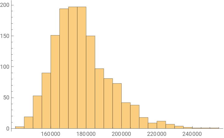
In the same way, visualizing the sample rates of audios.
In[]:=
sampleRate=AudioLength[Import[#]]&/@fileNames;MinMax[sampleRate]Histogram[sampleRate]
Out[]=
,
Out[]=
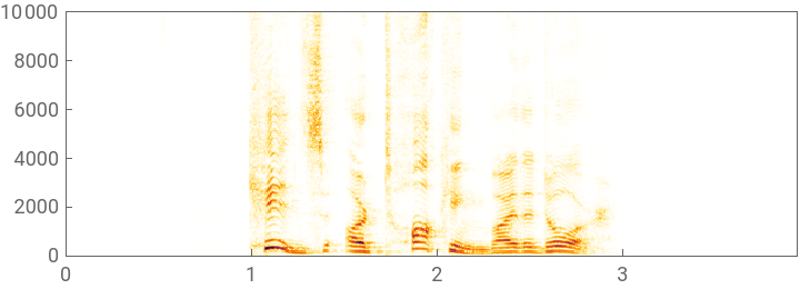
Visualizing the spectrogram of sample audio.
In[]:=
Spectrogram[Import[fileNames[[30]]]]
Out[]=
Dimensionality Reduction
Dimensionality Reduction
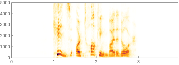
Now, it takes long time to run when we do augmentation in the training. Thus, we could reduce the dataset size reduction by resampling or removing unimportant information (silence). You could notice that the audio doesn’t seem natural, as they are recorded with sampling rate of 48khz. However, the voice band lies within 4kHz (low band) most of the times. Thus, to discard the unimportant information, we could resample it to12,000 Hz. We also need to compare their spectrograms, whether there is any major change. We need to be careful with the resampling, as it might affect the training. Thus, for now, we shall use this for experimental purpose. However, it has been used when training with the augmented data.
In[]:=
a= Import[fileNames[[30]]]AudioSampleRate[a]
Out[]=
Out[]=
Resampling the audio to 12kHz.
In[]:=
ane = AudioResample[a,12000];AudioSampleRate[ane]
Out[]=
The resampled audio
In[]:=
ane
Spectrogram of resampled audio
In[]:=
Spectrogram[ane,512,64]
Spectrogram of original audio
In[]:=
Spectrogram[a,512,64]Spectrogram[ane,512,64]
Out[]=
Out[]=
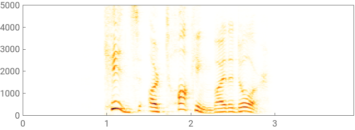
The spectrograms of both audios doesn’t vary that much. Still, we shall use this for experiment purpose, until we get the final results for comparison .
Silence removal
Silence removal
AudioInterval function is used here to visualize the silence periods in an audio. Silence removal is an another way to reduce the size of the dataset and reduce the training time eventually.
In[]:=
silence=AudioIntervals[Import[fileNames[[30]]],"VoiceInactivity"];AudioPlot[Import[fileNames[[30]]],Epilog{RGBColor[1,0,0,.5],Rectangle[{#〚1〛,-1},{#〚2〛,1}]&/@silence}]
Out[]=

Here, we could see that the 1s at the end and beginning of the audio is inactive. This is similar for other audios, also. Thus, it is safe for us to remove the 0.8 seconds at the end and beginning of the audios.
Create a new directory for preprocessed audio files without resampling
Directory without resampling
Data Grouping
Data Grouping
Now create a list of info about the dataset from the given filename . These are the file name identifiers that have been provided in the original dataset description.
Filename identifiers
Modality (01 = full-AV, 02 = video-only, 03 = audio-only).
Vocal channel (01 = speech, 02 = song).
Emotion (01 = neutral, 02 = calm, 03 = happy, 04 = sad, 05 = angry, 06 = fearful, 07 = disgust, 08 = surprised).
Emotional intensity (01 = normal, 02 = strong). NOTE: There is no strong intensity for the ‘neutral’ emotion.
Statement (01 = “Kids are talking by the door”, 02 = “Dogs are sitting by the door”).
Repetition (01 = 1st repetition, 02 = 2nd repetition).
Actor (01 to 24. Odd numbered actors are male, even numbered actors are female).
Sample data info
Gathering by the emotion types
Gathering by mean duration for each emotion . We could see that Calm and disgust has highest mean duration .
Feature Extraction And Data Augmentation
Feature Extraction And Data Augmentation
What are the features that better identify an emotion?
What are the features that better identify an emotion?
The features are used to train and tune a model to produce the desired output labels. A common issue faced is the choice of features. In general, it is not known which features can lead to the most efficient clustering of data into different categories.
An audio has mainly two kinds of feature: the physical features and the perceptual features. Physical features refer to mathematical measurements computed directly from the sound wave, such as the spectrum, the cepstral coefficient etc.,. Perceptual features are the emotional prosodic feature, which are subjective.
Lack of prosody knowledge can easily be perceived from the speech. Prosody can be viewed as speech features associated with larger units such as syllables, words, phrases and sentences. Humans use prosodic cues to express and understand the emotion in the natural language. Further, there are two types of prosodic features: Global and Local. Global prosodic features represent the statistics such as mean, minimum, maximum, standard deviation. Local prosodic features denote the temporal dynamics in the prosody
What are the feature extraction techniques that we are going to consider?
What are the feature extraction techniques that we are going to consider?
There are many feature extraction techniques available to extract the features . But we need to decide the features and feature extraction technique suitable for our task . For example, Zero-crossing rate which is the measure of number of times in a given time interval that the amplitude of the speech signals passes through a value of zero. It is mainly used to distinguish between voiced and unvoiced sounds (no vibration in vocal cord), classify percussive sounds. This may not be useful to classify an emotion. It would rather be useful to classify music genre or speech recognition tasks. Likewise, we need to choose the method based on their utility with respect to our task. Here, we have considered three feature extraction techniques here:
1
.Pretrained feature extraction
2
.Feature extraction based on Mel Spectrogram (deep learning)
3
.Pretrained Image classification network
Analysis of different ways of feature extraction
Analysis of different ways of feature extraction
Some insights can be gained by testing a large number of different features, combining different features into a common feature vector, or applying various feature selection techniques. The quality of the resulting manually crafted features can have a significant effect on classification performance.
Identification of the “best” acoustic features that characterize different emotions is a challenging task .The Munich Versatile and Fast Open-Source Audio Feature Extractor (openSMILE) allows the calculation of low- and high-level acoustic descriptors of speech. Still, identifying the best features is a problem, here .Thus, to eliminate the need of prior knowledge of best features, automatic feature extraction by neural networks is widely desirable.
The idea is to use an end-to-end network that takes audio as an input and generates a class label as an output. There is no need to compute features manually, nor to determine which parameters are critical for the classification. It is all done by the network itself. Namely, the network parameters are optimized during the training procedure to act as features efficiently dividing the data into the desired categories. But this sophisticated solution requires large labeled data-samples compared to conventional classification methods.
In many cases, only limited data is available for training purposes.The minimal training data problem, to a large extent, can be overcome by the method called as transfer learning. It uses an existing network pre-trained on extensive data to solve a general classification problem. This network is then further trained (fine-tuned) using a small number of available data to solve a more specific task. Pre-trained network parameters can be applied as features to train conventional classifiers that require lower numbers of training data
For simplicity, in this notebook, we shall use the RAVDESS data for experimentation
Experiment 1: Wolfram Audio (Transfer Learning)
Experiment 1: Wolfram Audio (Transfer Learning)
Here, Wolfram AudioIdentify V1 Trained on AudioSet Data is used as a pretrained featureExtractor Due to the availability of limited data, we are adopting the transfer learning approach to extract features from Audio. Moreover, it has been trained on the similar raw data, i.e. audio. Thus, the transferred features would be very much appropriate for our tasks.
Before doing the feature extraction, we need to create the dataset from filename identifiers . The dataset is created as an association between Audio file and Label. Other filename identifiers are not necessary for us in training.
Before doing the feature extraction, we need to create the dataset from filename identifiers . The dataset is created as an association between Audio file and Label. Other filename identifiers are not necessary for us in training.
Sub Experiment 1: With data augmentation
Why do we need data augmentation? This is also a technique to prevent the model from generalizing over the data (over fitting), which is more common when we have a small dataset . Dataset is usually done by increasing the amount of information in the samples or adding new synthetic samples. Here, we have tried two augmentation methods: on the raw data (waveform) by shifting its frequency and shifting its time; and on the log MEL spectrogram by time warping.
1) Raw data augmentation
1) Raw data augmentation
Here the raw data (audio) is augmented by shifting the frequency and stretching the time. But if we view the performance of the model, it would be evident that this might not be a better method and also it requires careful consideration on how much augmentation that we need to do.
Save it in a different directory . (resampled and augmented data)
2) Mel Spectrogram Image Augmentation (see Experiment 2)
In this method, we are directly applying the augmentation to the log MEL spectrogram of the audio, by modifying some of the pixels . See experiment 2.
3) Shift Augmentation using NetEncoder in the featureExtractor (pretrained) (experiment with this after the getting the initial results of net gradients)
3) Shift Augmentation using NetEncoder in the featureExtractor (pretrained) (experiment with this after the getting the initial results of net gradients)
Sub Experiment 2: Without data augmentation
Sub Experiment 2: Without data augmentation
Here, we have not implemented any of the data augmentation methods . We just directly defined the pretrained feature extractor model .
Define the feature extractor model
Now, we need not have the classification layer of the pretrained model and the output shape needs to match ours. Thus,we are truncating upto 3 layers from below.
Now, we need to apply the feature extractor to all the samples present in our dataset.
How many features are there?
Experiment 2: Using feature Extractor function(Audio Mel Spectrogram)(with data augmentation)
Experiment 2: Using feature Extractor function(Audio Mel Spectrogram)(with data augmentation)
After training the model without data augmentation, when we mapped the gradients into the spectrogram, it is evident that it learns from the areas where the features are not there . So, we have extracted the NetEncoder function and designed the encoder based on the parameters of that function . The augmentation technique is encoded in the encoder function itself .
Experiment 3: Transfer Learning on Audio Mel spectrogram image
Experiment 3: Transfer Learning on Audio Mel spectrogram image
Here, the MEL spectrogram image is passed as the input and feature knowledge is enhanced using ResNet 50 pretrained model. See the Training section’s Experiment 3.
Defining and Training the Model
Defining and Training the Model
Now, as we have extracted the features, we could define and train the model .
Experiment 1: Using the features extracted in the simple RNN model (without data augmentation)
Experiment 1: Using the features extracted in the simple RNN model (without data augmentation)
Define training data and testing data . This is a simple gated recurrent layer with kernel size 128. Early stopping is included in the training phase to prevent overfitting. Here, the data has been split into 3 parts: train, test and validation (8% of the train data). Test data will be used during the evaluation phase, as an unseen data. It cannot be considered totally unseen, as it is similar in many characteristics with train and validation data.
Train the network
The accuracy is 62 %, which is comparatively better. If we could include data augmentation, it might work better.
Experiment 2: Using the features extracted in the simple RNN model (with raw data augmentation)
Experiment 2: Using the features extracted in the simple RNN model (with raw data augmentation)
Define training data and testing data . This is the same RNN model as the previous. But we need to run it with the augmented raw data.
Train the network with the augmented data
The result is very much worse . Maybe, we have augmented a lot or the raw data augmentation may not be good method to improve the performance .
Experiment 3: With simple CNN model
Experiment 3: With simple CNN model
Convolutional Neural network may not be appropriate due to the size of the dataset . But for experimental purposes, we shall try with the simple CNN layer . Here, the audios are encoded as AudioMelSpectrogram and they are converted into grayscale image . Then, they are fed into the CNN . This is very much like an image classification.
Due to the small size of the dataset, simple CNN is not very much apt for training .
Experiment 4 : With CNN and Transfer Learning
Experiment 4 : With CNN and Transfer Learning
This is similar to the image classification network with the use of pretrained model (transfer learning) . The basic idea of transfer learning is: obtain a model trained on a large dataset and transfer its knowledge to a smaller dataset. We freeze the initial convolutional layers of the network and only train the last few layers which make the classification/prediction. The convolutional layers extract low - level features and the later layers identify specific features within an image.
Thus, we can use a network trained on unrelated data and apply it to our task as the low level features are mostly common and universal.
Thus, we can use a network trained on unrelated data and apply it to our task as the low level features are mostly common and universal.
Take the convolution layer from the pretrained model and attach the new classification layer
Comparatively, Transfer learning works better than the CNN built from scratch. Still, the pretrained audio feature extractor performs well when it comes to extracting the right features. The reason is the dataset is not similar here and the ResNet is trained on images, while Wolfram audio detection feature extractor was trained on audio. Thus, here, the features are transferred poorly.
Exploring the “best” features
Exploring the “best” features
Now, we need to calculate the gradients of the trained network and map it into the MEL spectrogram to know what are the features that it is considering to recognize the emotion.
Combine the feature extractor and trained net .
Take one sample audio
Now, calculate the gradient .
There are three spectrograms for that audio. Highlight the areas that indicate emotions .
Now, if we could see, the network learns from where there are no emotional features . This means, network has learnt to recognize emotion somehow, without properly learning . Thus, we shall experiment again with the data augmentation .
Train again with the new classifier with augmentation added . We shall join the feature extractor and classifier here. So we could directly give the raw data for training.
featureNet2 is the feature extractor with data augmentation encoding .
Emotional Subtitling
Emotional Subtitling
Now, we have got the output of emotion, I have done a very simple annotation here . But in the future, we could create an interface for that to display the emotion in form of emoji or in the colored text, along with the spoken text . I considered the ASCII standard of emojis, using emoji data repository from Wolfram data repository and concatenated it as an emoticon with the spoken text, for the corresponding recognized emotion.
This is a very very simple output , concatenating the emoticon with the recognized speech .
Concluding remarks
Concluding remarks
In this project, various ways of augmentation, feature extraction and learning methods are experimented . From the transfer learning approach with data augmentation, the accuracy of 73.4% could be achieved. The major issue here is the size of the dataset available. As the current benchmark datasets are comparatively small, we could increase the training of the model if we annotate more data.
Second thing is, we have only considered the pitch level prosodic cues, based on MEL spectrogram. But, the global and local prosodic features extracted from words
and syllables would help to analyze the contribution of different segments such as sentences, words and syllables and their positions in the utterance toward
emotion recognition. This could be included in our future work. We could even use this to analyze what kind of features contribute a lot: global or local?
Thirdly, this SER is built upon English Language. It would be interesting to learn what kind of features are critical in multilingual dataset. Building an SER system whose prosodic feature analysis is independent of language would be great to have.
Finally, in the future progress, we could integrate SER with speech recognition and embed it in a video streaming interface, where we could animate the closed captions based on the emotional information in a visually pleasant way. This could make it as a good application for people with hearing impairment issues and increase user experience satisfying the universal usability of the video streaming application.
Keywords
Keywords
◼
Speech Emotion Recognition
◼
Emotional Prosody
◼
Transfer learning
◼
Emotional Subtitles
◼
Convolutional Neural Network
◼
VGG
◼
RESNet-50
Acknowledgment
Acknowledgment
I express my gratitude to the entire team who organized this summer school in an exciting and organized manner. I sincerely thank my mentor, Markus Van Almsick in supporting and teaching me , all along the project. This is the first time I am working on neural networks, using Wolfram Language. With the guidance of my mentor, I have got to learn various applications and usage of Wolfram Language in the neural networks. I also thank Stephen Wolfram for the suggestion of the project idea and his duly monitoring over the progress of our projects.
References
References
◼
Schuller, Björn W. “Speech emotion recognition: Two decades in a nutshell, benchmarks, and ongoing trends.” Communications of the ACM 61.5 (2018): 90-99.
◼
Park, Daniel S., et al. “Specaugment: A simple data augmentation method for automatic speech recognition.” arXiv preprint arXiv:1904.08779 (2019).
◼
The Ryerson Audio-Visual Database of Emotional Speech and Song (RAVDESS). https://zenodo.org/record/1188976
◼
Surrey Audio-Visual Expressed Emotion (SAVEE) Database. http://kahlan.eps.surrey.ac.uk/savee/