This is a joint work byAntonín Slavík, Charles University, Prague, Czech Republic; slavik@karlin.mff.cuni.czStan Wagon, Macalester College, St. Paul, Minnesota, USA; wagon@macalester.edu
Back in January 1990 Wolfram Research organized the first Mathematica conference, in Redwood City, California. The conference banquet was held at San Francisco's Exploratorium and there Leon Hall (Univ. of Missouri, Rolla) and Stan Wagon saw a model of a square wheel rolling smoothly on a certain bumpy road. This was completely new to them, so later that evening they borrowed a computer and exercised their mathematical and Mathematica'l skills to work out the geometry of the construction and make an animation of a square rolling along a sequence of catenaries. That led to some interesting large models: first a full-size tricycle that can be ridden smoothly on a 25-foot road, and more recently a 26,000-pound bridge that can be rolled, by hand, so that boats can pass underneath it. The ideas underlying this bridge design are so radical, nontraditional, and elegant that the bridge won the Bridges Design Award for 2022 [11].
Another consequence of this story is that the bike at Macalester College, which has been in storage for ten years, is now being brought back out for a day or two each year.
Figure 1. In April 2023, many students at Macalester College came to an event that displayed the square-wheel tricycle designed by Stan Wagon.
An Elegant Differential Equation
An Elegant Differential Equation
Initialization code
Suppose a wheel is given in polar coordinates as , with the origin viewed as the center of mass, and the corresponding road (i.e, the road on which the wheel will roll—we assume friction prevents any sliding—with the center of mass moving neither up nor down) is ; see Figure 1 and note that is negative. Let be the polar angle defining the point that will touch the road at .
r=r(θ)
y=f(x)
y
θ(x)
x
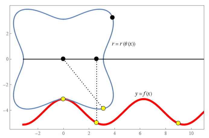
Figure 2. The relationship between a wheel and the corresponding road. Here the road is and the wheel’s polar form is .
cos(x)-
17
r=
17
-9+(2θ)
17
-82
tan
9+(2θ)
17
+82
tan
We have the radius condition: . And matching the arc length of the road to the relevant part of the perimeter of the wheel (using the polar coordinate arc length formula) leads to +α. We can use the radius condition and differentiation of this equality to get the arc length condition: . And that leads to the simple and elegant differential equation =, with initial value . This can all be automated using differentiation and as follows.
f(x)=-r(θ(x))
x
∫
0
1+
t=2
(f(t))
∂
t
θ(x)
∫
-
π
2
2
r(α)
2
(r(α))
∂
α
1+=+
2
[(θ(x))(x)]
′
r
′
θ
2
θ
x
2
r(θ)
2
r
θ
θ
x
1
r(θ(x))
θ(0)=-
π
2
Solve
In[]:=
Solve+α,θ[x],Reals,Assumptions->r[θ[x]]>0
∂
x
x
∫
0
1+
t2
((-r[θ[t]]))
∂
t
θ[x]
∫
-π/2
2
r[α]
2
(r[α])
∂
α
∂
x
Out[]=
[x]
′
θ
1
r[θ[x]]
The road is then where is the solution to the differential equation. Because θ is an increasing function of , it has an inverse which satisfies =r(θ); this can be solved by the definite integral . The result must then be inverted to get . For more on these formulas, and variants in the case that the wheel is given in a different form, see [2, 6, 7, 8, 9, 10].
y=-r(θ(x))
θ(x)
x
x(θ)
x
θ
x=r(t)t
θ
∫
-π/2
θ(x)
Here we always take the polar center of the wheel to be . It might happen that this point is not inside the wheel. Later we will see the importance of a wheel that is a circle some distance from the origin. Or the wheel might be simply a straight line.
(0,0)
The Catenary Road for a Straight Line
The Catenary Road for a Straight Line
If , the wheel is a circle, , and the road is the straight line . But if , then the wheel is a straight line (here ) and the road turns out to be the catenary . The intermediate equations relating θ and are and . Here is how to solve the differential equation and obtain the road in one line.
r(θ)=1
θ(x)=x-
π
2
y=-1
r(θ)=-cscθ
-π<θ<0
y=-coshx=(+)
1
2
x
-x
x
θ=-2()
-1
cot
x
x=-ln-tan
θ
2
In[]:=
ExpToTrigTrigExpandCsc[θ[x]]/.DSolve[x]Csc[θ[x]]-1&&θ[0]-,θ[x],x1
′
θ
π
2
Out[]=
-Cosh[x]
Here is how to get all the relationships from a solution to the differential equation.
In[]:=
r[θ_]:=-Csc[θ];θFunc=θ[x]/.DSolve[x]r[θ[x]]1&&θ[0]-,θ[x],x1Simplify[x/.Solve[θθFunc,x,]〚1〛,-π<θ<0]/.Log[z_]Log-ExpToTrig[TrigExpand[-r[θFunc]]]
′
θ
π
2
1
z
Out[]=
-2ArcCot[]
x
Out[]=
LogTan
θ
2
Out[]=
-Cosh[x]
Here are the same results, using the definite integration formulation (the assumption on ρ is needed for the integration).
In[]:=
xLine=Assuming-≤ρ<0,r[θ]θ/.ρθθFunc=FullSimplify[θ/.Solve[xxLine,θ]〚1〛,x∈Reals]/.0ExpToTrig[TrigExpand[-r[θFunc]]]
π
2
ρ
∫
-
π
2
1
Out[]=
-Log-Tan
θ
2
Out[]=
-2ArcCot[]
x
Out[]=
-Cosh[x]
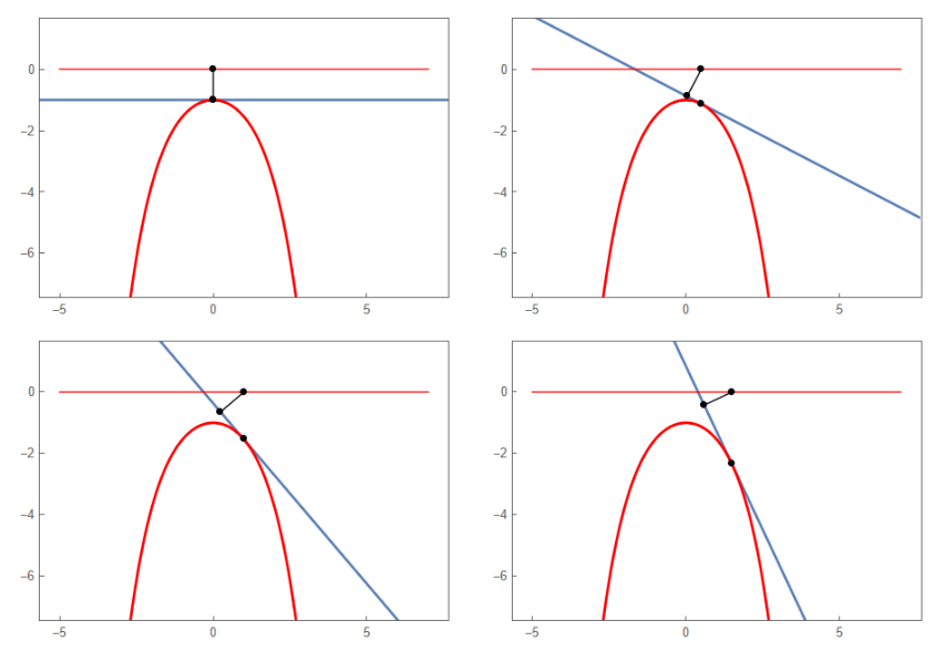
Figure 3 shows an infinite line rolling along a catenary. The "center" of the line — the point — moves along the -axis. Remarkably, this relationship was discovered by James Clerk Maxwell: in February, 1849 (he was 18 at the time) he published a paper [3] with many examples of rolling wheels. Maxwell’s example 12 [3, p. 537] says
(0,0)
x
"The straight line whose equation is , rolled on a catenary whose parameter is , traces a line whose distance from the vertex is ."
r=asecθ
a
a
A Square Wheel
A Square Wheel
Figure 4. A square rolls on inverted catenaries.
Figure 8. A demonstration that illustrates several road–wheel relationships. An additional case of a “4-loop sawtooth” can be found in the full demonstration here https://demonstrations.wolfram.com/RoadsAndWheels/.
The Cody Dock Bridge
The Cody Dock Bridge
Figure 14. This demonstration allows one to change the amount of rounding at the corners of the square.
Triangular Difficulties
Triangular Difficulties
Figure 19. A demonstration for rolling triangles, squares, pentagons, and hexagons.
Conclusion: The Perfect Catenary
Conclusion: The Perfect Catenary
References
References
12. Exploratorium, Square wheels, https://www.exploratorium.edu/snacks/square-wheels and https://www.exploratorium.edu/exhibits/square-wheel.
CITE THIS NOTEBOOK
CITE THIS NOTEBOOK
A Rolling Square Bridge: Reimagining the Wheel
by Stan Wagon and Antonín Slavík
Wolfram Community, STAFF PICKS, May 9 2023
https://community.wolfram.com/groups/-/m/t/2917199
by Stan Wagon and Antonín Slavík
Wolfram Community, STAFF PICKS, May 9 2023
https://community.wolfram.com/groups/-/m/t/2917199