Lattice gas automata provide a discrete approach to fluid simulation, where continuous fluid properties appear emergently. In this project, I investigated methods to write optimized implementations of a triangular lattice fluid cellular automaton and explored applications of modern hardware acceleration for this problem.
The Wolfram Fluid CA Model
The Wolfram Fluid CA Model
Theory
Theory
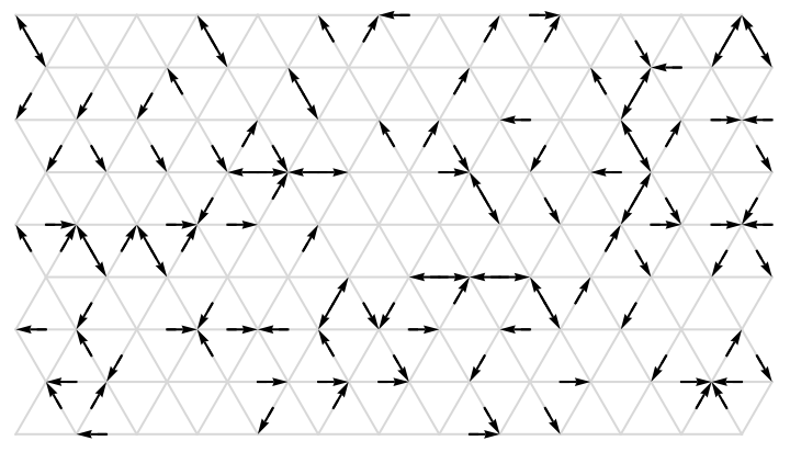
Most of the work in fluid dynamics has taken a macroscopic approach of describing fluid systems as a continuum process through differential equations. While this approach provides high accuracy results, the numerical solutions used in these techniques require a large number of floating point operations and provide little insight into the origin of the macroscopic dynamics. Behavior such as wave propagation in the density field or diffusion in the velocity field are written explicitly in the equations of motion despite these behaviors being emergent in real systems. One simplified class of models used to understand this emergent behavior are lattice gas automata. Lattice gas automata simulate the discrete motion of virtual fluid elements, whose motion is restricted to a lattice.
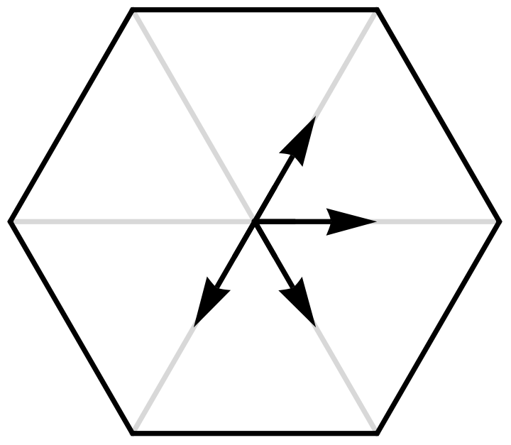
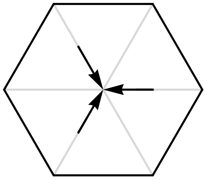
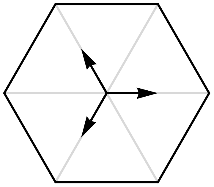
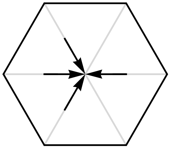
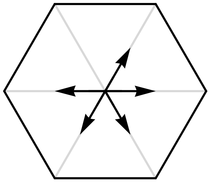
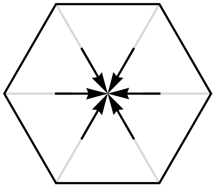
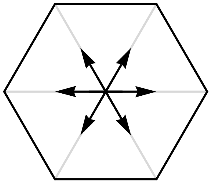
In this triangular grid fluid automaton, the fluid elements move on a triangular grid. At a vertex, they are able to collide with other fluid elements. In many of the collision rules, the fluid elements simply move through each other. This is often required to remain number and momentum conserving on a discrete grid. Where possible, interactions are added by rearranging collisions that have multiple momentum conserving configurations. All complex interactions either have at least one pair of fluid elements opposite to each other, or have three fold symmetry.
In[]:=
MapIndexed[fluidCellRuleGraphic[#,Reverse[RotateRight[#,<|1->3,2->3,3->3,4->3,5->3,6->4,7->0,8->2,9->3,10->0,11->3,12->4,13->3,14->3|>[First[#2]]],<|1->2,2->2,3->2,4->2,5->2,6->2,7->1,8->1,9->2,10->2,11->2,12->2,13->2,14->2|>[First[#2]]]]&,First/@GatherBy[Tuples[{0,1},6],Sort[Permute[#,CyclicGroup[6]]]&]]
Out[]=
,,,,,,,,,,,,,
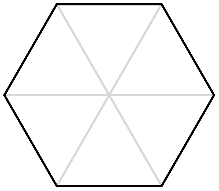

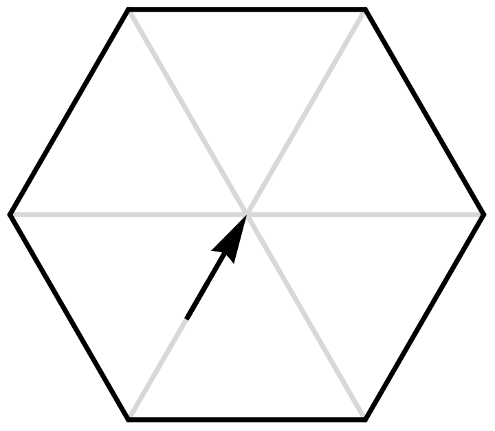
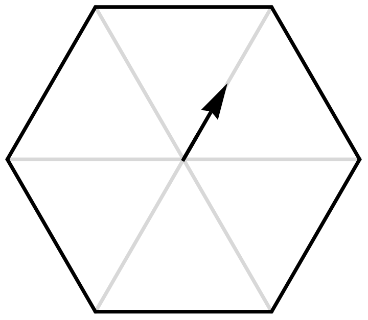
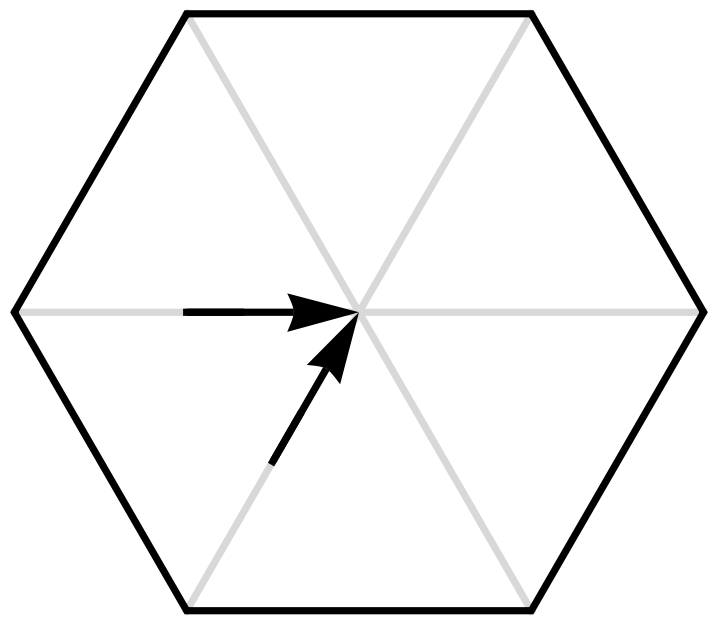
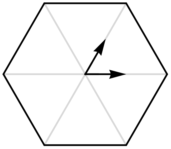
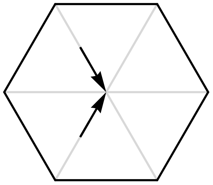
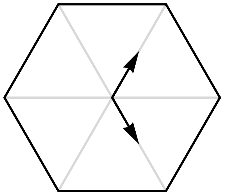
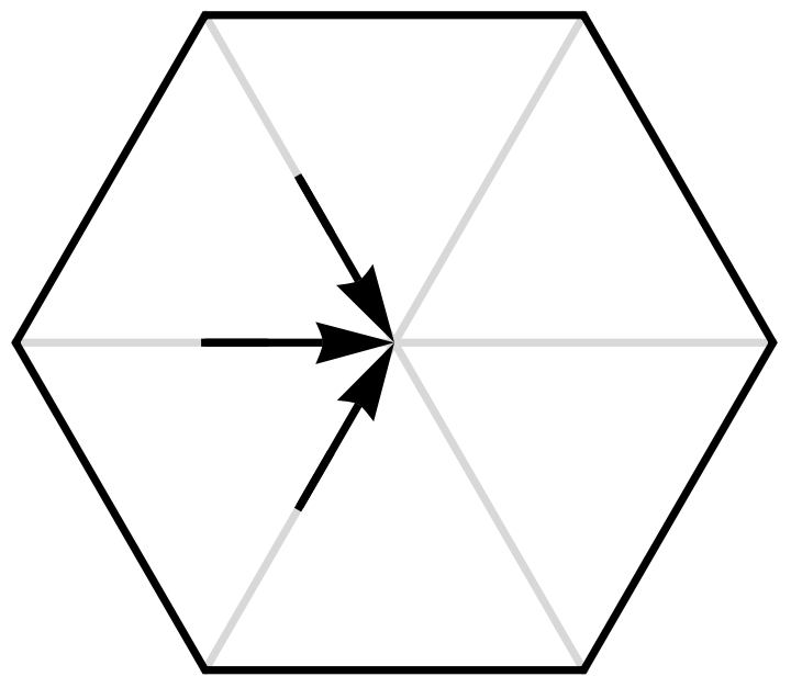
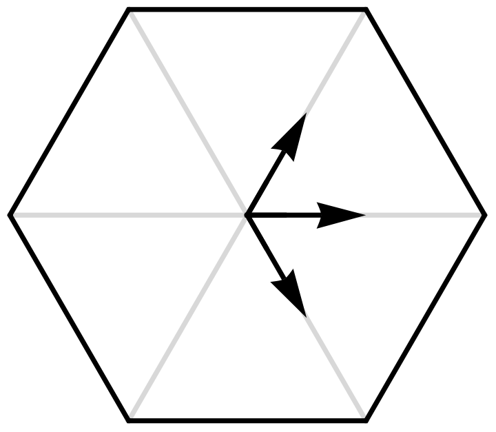
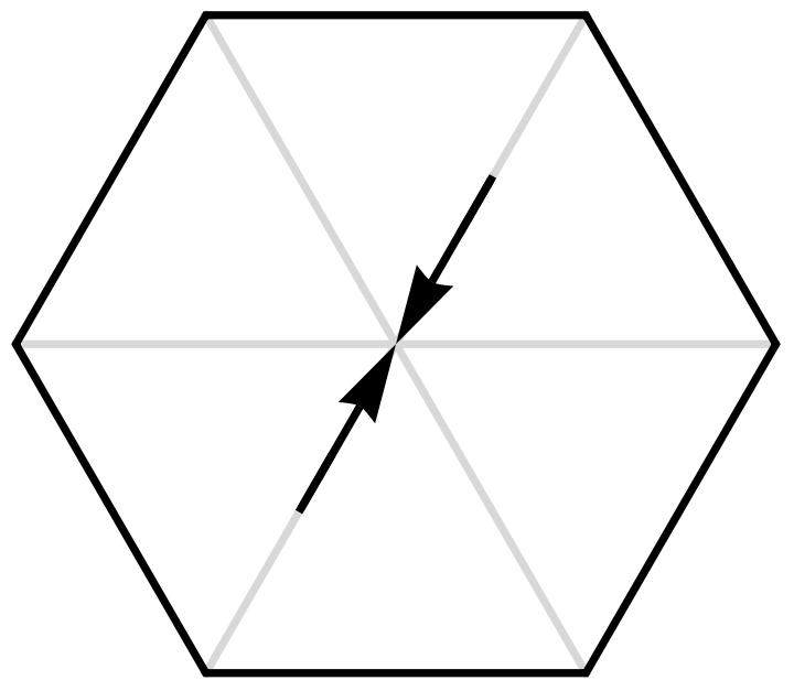
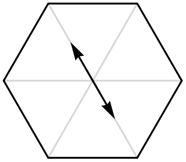
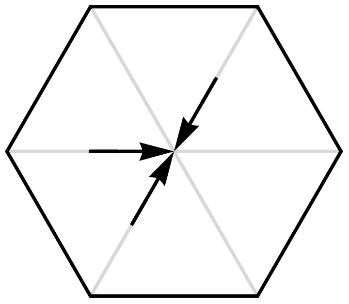
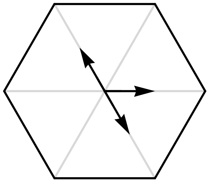
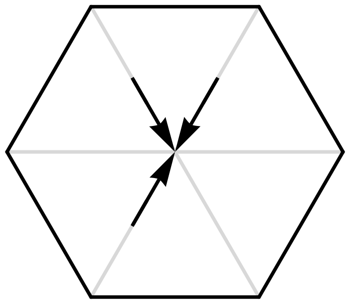
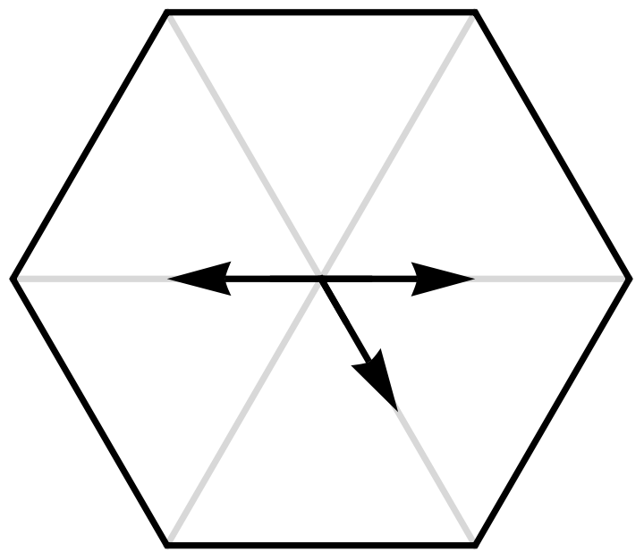
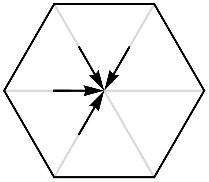
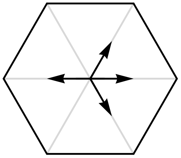
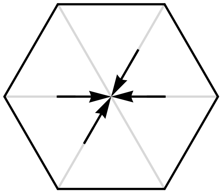
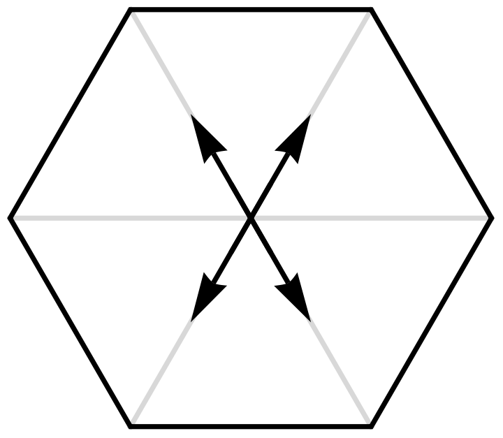
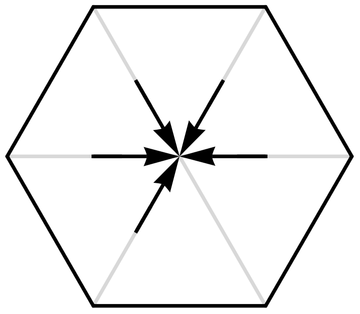
Standard and Existing Implementations
Standard and Existing Implementations
The results of the original simulation are documented on pages 378-380 of A New Kind of Science [1], but the source code is not published and is not written in the Wolfram Language. One public implementation is available as a Wolfram Demonstrations project [2]; this implementation uses a cellular automaton, but the rule set is very obscure, and the cells take values of 0-63, which is not a simple way to describe the ground truth of the model.
Finding a Simpler Model
Finding a Simpler Model
Perhaps surprisingly, the fluid elements on this triangular lattice accommodate an array encoding scheme. The ability to perform this encoding follows from each edge holding two locations for fluid elements, allowing for the horizontal edge of each triangle to be partitioned into two cells. This aligns well with the other two edges of the triangle, since they follow a bilateral symmetry. This is quite fortunate, as it allows for the individual fluid elements to be assigned to a coordinate on the grid, which corresponds to a location on the lattice and a direction of travel.
In[]:=
Show[meshIntersection[triMesh2[ArrayMesh[ConstantArray[1,{10,14}]]],Rectangle[{-0.01,0},{9.5,12}]],Graphics[{Transparent,EdgeForm[Thick],GeometricTransformation[ArrayMesh[ConstantArray[1,{31,19}]],ScalingTransform[{1/2,Sqrt[3]/6}]@*TranslationTransform[{0,-0.5}]]}]]
Out[]=
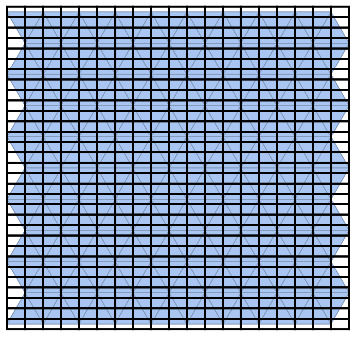
With a sufficient rule specification, it should be possible to use this underlying structure to exactly reproduce the behavior of the lattice gas over a rank 2 array.
The Block Automaton
The Block Automaton
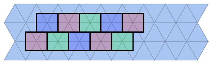
To implement the rules over this array, it is most natural to use a block cellular automaton. Unlike the traditional cellular automaton models which use a kernel to update an individual cell, block automatons divide the array of cells into blocks and perform a replacement rule on each block. Because this operation is local to each block, the partition scheme needs to be moved on every other step.
Collision Step
Collision Step
As applied, the collision rule is local to each vertex. The region around each vertex consists of 6 cells.
Out[]=
Transport Step
Transport Step
On the outbound step, the fluid elements need to be moved towards the next vertex in the direction of travel. To perform this operation, the blocks need to lie between the vertices.
Out[]=
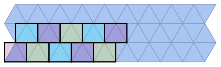
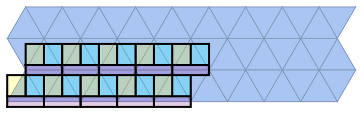
The operations performed by the blocks are localized across each edge. The possible rules along each edge are compiled to a larger rule for each block, so that the transport step can use the same partition size as the collision step. It should be noted that there is more than one valid way to construct the transport rule, depending on the partition scheme.
Out[]=
Bulk Behavior
Bulk Behavior
In[]:=
FoldList[mergePartitions[If[#2==1,collisionPartition[#1]/.collisionRules,transportPartition[#1]/.transportRules]]&,SeedRandom[37];Reverse[RandomChoice[{0.8,0.2}->{0,1},{25,25}]],Array[Mod[#,2,1]&,100]]
In[]:=
MapThreadfluidAutomatonPlot,,Array[Mod[#,2,1]&,100+1]
In[]:=
ListAnimate,ControlPlacement->Bottom
Out[]=
In[]:=
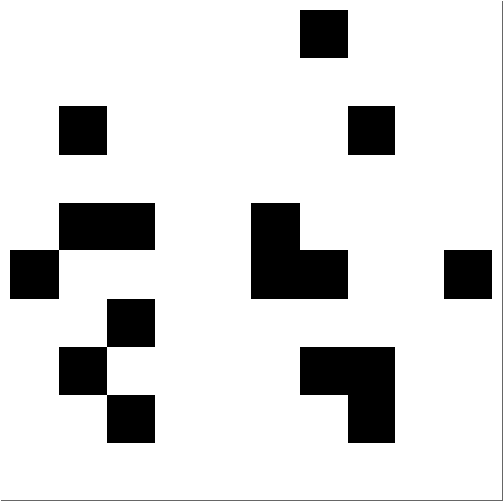
MapArrayPlot,

In[]:=
ListAnimate,2,ControlPlacement->Bottom
Out[]=
Boundary Conditions
Boundary Conditions
With the bulk implementation, we get quite lucky as a side effect of the ReplaceAll function. Since the blocks near the walls are padded with Null values, no pattern in the set of bulk dynamics patterns will match the block, and the block will effectively skip a step. When a step is skipped in this manner, the fluid element is implicitly rotated by 180 degrees, as it now occupies a cell which will be transported in the opposite direction. This can be seen as a good thing, as it ensures that the simulation is bounded and local. However, we would expect particles to reflect off of walls instead of coming back in the opposite direction of travel. New rules need to be specified at the boundary to fix the default behavior.
At a minimum, we would like to have a well specified boundary at the boundary of the array (the computation domain).
For now, since arrays in the wolfram language are not typed, boundary conditions will be specified using strings placed in the array at the boundary. Because for now the boundary is only rectangular, most of the boundary conditions can be described by a small set of boundary rules to demonstrate some basic reflections.
Walls
Walls
With the current scheme, a full description of the wall dynamics (assuming that particles cannot occupy walls) would raise the rule set from 64 rules to 729.
It is not clear what solution would work best to generalize the wall behavior. It is open question whether discrete surface normals can be calculated and used to find the correct permutation of a block, or even whether a single set of rules will be visually consistent with the true angle of the wall.
An example set of reflection rules for walls can be written manually.
Sources
Sources
The simplest implementation of a source will spawn a new outbound fluid element at every step.
Generating a stream of fluid elements in this manner without any random perturbations in the velocity might not simulate realistic fluid behavior, or could be analogous to supersonic flow. While the use of a stochastic method for spawning fluid elements would be nondeterministic, nondeterministic rules could be reasonably implemented using a RuleDelayed statement, which make a random decision at every step.
Sinks
Sinks
We expect sinks to remove fluid elements from the simulation. Fluid elements could either be removed when they are next to a sink or removed when they collide with a sink. In some configurations, all adjacent fluid elements in a block necessarily collide with a sink, and vice versa. The simplest general implementation would be to remove all fluid elements that share a block with a sink on both steps.
Visualization
Visualization
Given the nature of the standard grids used for visualization, it makes sense to use mesh regions as they can efficiently store a list of connected components. While the Wolfram Language can generate graphs with triangular tessellations, there are no built in functions to generate a mesh with a regular tessellation of triangles. The most similar function is ArrayMesh, which generates a mesh of squares in a similar manner to ArrayPlot.
A triangular lattice can be generated by dividing a rhombic tessellation, which can be made using a shear transformation.
Thankfully, all of the squares generated from ArrayMesh have the same vertex order, which makes it straightforward to cut them into triangles.
These operations can be folded into a function:
To operate on a rectangular array, the mesh should be cut down.
These operations are also folded into a function.
The fluid elements should be aligned to the mesh.
Using graphics transforms, the underlying array can also be displayed with ArrayPlot and aligned to the mesh.
Writing a Performant Model
Writing a Performant Model
Implementation with the Compiler (FunctionCompile)
Implementation with the Compiler (FunctionCompile)
The Wolfram language primarily performs computation through symbolic manipulation. While this method of computation is very versatile, it is known to be slow both on the frontend and the backend. One option is to write the algorithm using static types, and compile down using FunctionCompile. FunctionCompile has restrictions on which Wolfram language functions are supported, and on which data types are supported. It can also be more difficult to fix not implemented errors, or obscure type conflicts. In my attempt at writing an algorithm which could be compiled down, I decided to use a rank 2 array of machine integers, and partition it down to a rank 4 array before performing the replacement rule and merging it back up to a rank 2 array. To maintain a static footprint and avoid unimplemented functionality, the array is rotated instead of padded to offset the partition grid. Some implementation errors also occurred when trying to use associations for the rules; instead, they were hard coded as a rank 6 array.
Bitwise Block Automata
Bitwise Block Automata
Since CPUs are well optimized to perform bitwise operations, bitwise implementations of 1D cellular automata have been explored previously to accelerate performance. While these bit vectors work well on 1D arrays, bit arrays are not currently implemented in the Wolfram language. One alternative is to instead use a list of integers.
To evaluate a block automaton in a bitwise fashion, the most straightforward way to extract the local information of each block is by using a series of bit masks.
Concluding Remarks
Concluding Remarks
This work demonstrates an array based technique for evaluating lattice gas automata on triangular arrays. This technique is simpler and more fundamental than standard techniques used for this lattice gas automaton. Future work needs to be done to explore optimization techniques and system dynamics.
Acknowledgments
Acknowledgments
I would like to thank Dr. Stephen Wolfram for his assistance in providing project direction. I would like to thank my mentors Piero Sanchez and Robert Nachbar for their active assistance in my project. I would like to thank Dugan Hammock and Daniel Sanchez for taking the time to meet with me about some details of my project.
References
References
1
.S. Wolfram (2002), A New Kind of Science. Wolfram Media.
2
.E. Zeleney (2009), “Cellular Automaton Fluids,” Wolfram Demonstrations Project. https://demonstrations.wolfram.com/CellularAutomatonFluids/.
Cite This Notebook
Cite This Notebook
Optimizing the Wolfram Fluid Cellular Automaton for Modern Hardware
by Joseph Stocke
Wolfram Community, STAFF PICKS, July 9, 2025
https://community.wolfram.com/groups/-/m/t/3496427
by Joseph Stocke
Wolfram Community, STAFF PICKS, July 9, 2025
https://community.wolfram.com/groups/-/m/t/3496427