Wolfram Cloud Document

CITE THIS NOTEBOOK: The Effects of Dimensions D!=3 on Galactic Rotational Velocity Curves by John Blakely. Wolfram Community JAN 13 2023.

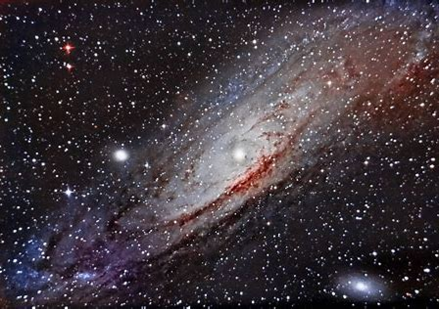
In this project , we explore the effect of variable dimensional discrete space on galactic rotational velocity curves. We have found that, due to the nuances introduced by extrapolating the physics to fractional dimensional space, accurately expressing the rotational velocity in this discrete space requires a more careful analysis than what was possible in this project. Beyond this, we were able to reach an expression for the Newtonian Gravitational Potential, by extending the well explored hypothesis of Modified Newtonian Dynamics (MOND) [1,2] to Hausdorff Dimensional Space [3, 4, 5, 6]. With this expression, we explored the effect of a local dimension perturbation on the scalar potential. We conclude that, in some cases, the perturbation could flatten the potential enough to possibly create the observed galactic rotational velocity curves. However, our conclusion comes with several caveats that could very well carry non-negligible effects that will require further analysis in future projects.

1. Introduction2. Gravitational Potential in D Dimensions3. Galactic Rotation Curves in the Scope of the Wolfram Physics Project 3.1. Rotation Curve on a Regular Grid Graph 3.2. Inducing Dimension Perturbations 3.2.1. Radial Perturbations 3.2.2. Vertex Specific Perturbations4. Conclusions 4.1. Future Work 4.2. Outlook

1. Introduction

In 1983, an Iranian physicist Mordehai Milgram [2] hypothesized that, instead of dark matter, modified gravity actually answers the missing mass problem. Since then, there are number of observations that disprove modified models of gravity, such as the Matter power spectrum, Baryonic Acoustic Oscillations, etc. [7,8]. However, modified gravity has had massive successes in predicting the rotational velocities of galaxies. But if there existed modified gravity, could it be a tell-tale sign of discrete spacetime? In this project we explore whether the rotational velocity curves in galaxies could imply a discretized spacetime, as described in the Wolfram Physics Project.

2. Gravitational Potential in D Dimensions

To understand the shape of the gravitational potential in galaxies in D ≠ 3 spacetime, we follow the derivation presented by [9]. It begins by defining the integral of a spherically symmetric function f(r) over a fractal metric space W with a Hausdorff measure μ [10]. This is expressed as

∫

fdμ



Γ



∞

∫

f(r)

D-1

where Γ is the Gamma Function and D is the Hausdorff dimension measure. The Hausdorff measure μ [10] can be thought of as the equivalent to taking a sphere on a spacetime manifold described by the metric space W and finding its equivalent volume. This measure gives an indirect notion for the dimension D of the graph-spacetime.

With this expression for the volumetric integral in D space, we can now use [9]’s expression for Gauss’s Gravitational Law

(D)

-|g

D-1

∫

to reach (see [9] for the full derivation) the expression for the gravitational potential:

Φ(r)-

1-D/2

Γ

G

(D-2)

∫

ρ(r)

D≠2

and

Φ(r)

∫

ρ(r)

D2

,where G is Newton’s gravitational constant,

is the scale factor, and ρ(r) is the mass distribution.Now with the gravitational potential defined, we now need to understand the mass distribution in fractional dimension space. For ease, we assume that, in D=3 space, the baryonic component of galaxies is best fit by the Plummer Mass Distribution [11], defined as

ρ(r)

4π

where M is the mass of the galaxy and b is the Plummer Radius, or the radius of the central core. Now, to extend the Plummer Model to non-integer dimensional space, we again follow [9] by rescaling the radius and the Plummer radius by the scale factor

ρ(r)

4π

With this, the equations for Φ becomes

Φ(r)

1-D/2

Γ

GM

2π(D-2)

∫

D≠2

and

Φ(r)

3MG

4π

∫

D2

With this we are now able to extend the analysis to the graphs in the scope of the Wolfram Model.

3. Galactic Rotation Curves In the Scope of the Wolfram Physics Project

Defining fundamental physics in terms of a hypergraph, and in turn discrete, representation of spacetime, allows for the addition of the spatial dimension as a free parameter. Whether or not there is reason to expect the spatial dimension to change, either locally or globally, on large scales is still unclear, but since it is allowed in General Relativity and some scenarios in Quantum Field Theory [12], there isn’t any obvious reason for it to not happen. However, the means by which dimension could be perturbed is not understood if possible. In the case that spatial dimension could be variant, the Wolfram Physics Project [5] could be a candidate model for describing fundamental physics. In this project, we proceed forward assuming that the machinery of the Wolfram Physics Project is true.

3.1 Rotation Curve on a Regular Grid Graph

To begin, we write the functions, described in Section 2, in Mathematica.

(************PlummerMassDistribution**************)ρ[r_]:=((3*M)/(4*π))*((1+((r^2))))^(-5/2)(************ScalarPotentialFunction**************)(*Integral(Usingdummyvariablesy=rands=D)*)integral[y_,s_]:=ResourceFunction["FractionalIntegrate"][ρ[y],{y,s}](*IntegralCoefficient*)intcoef[r_,D_]:=If[D==2.,2/(l^2),((2*(π^(1-(D/2)))*Gamma[D/2]*G*(l))/(D-2))](*ScalarPotential*)ϕ[r_,D_]:=intcoef[r,D]*integral[r,D]

We make the non-negligible simplification of setting all constants to 1 because it isn’t understood how these constants will be defined in The Project.

(********************Constants********************)(*Newton'sGravitationalConstant*)G=1(*MilkyWayMass*)M=1(*PlummerRadius*)b=1(*ScaleLength*)l=1

The next step is to define a grid graph to model spacetime in the Wolfram Physics Model.

In[]:=

(******************GridCreation*******************)(*ActualGrid*)grid=GridGraph[{11,11},ImageSize400,VertexSize0.6`,VertexShapeFunction"Circle"](*CenterofGrid*)center=GraphCenter[grid]

Out[]=

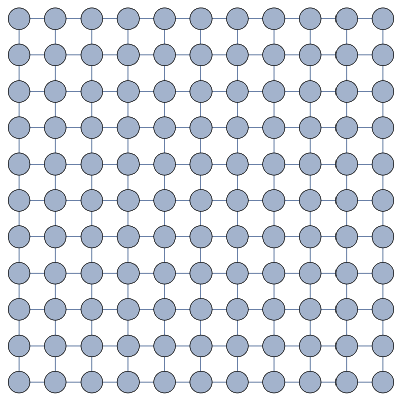
Now with this graph, we have to define both a measure of distance and the Hausdorff dimension. Sparing all of the measure theoretic details of the method, we define the dimension at each vertex as the dimension created by a sphere, on the grid manifold, with a radius of one edge length. We also define the distance on this manifold as the edges needed to transverse between vertex

and

. In Mathematica, this is

(*************MeasurementsontheGrid**************)(*Dimensions*)dim[r_,g_]:=ResourceFunction["WolframHausdorffDimension"][g,r,1](*Distance*)GraphDistSmooth[g_,v1_,v2_]:=If[String[v1]===String[v2],1,GraphDistance[g,v1,v2]]

With methods to measure distance and dimension, we are able to use the methods from [9] presented in Section 2. To do this, we use the techniques implemented by [12] to color the grid manifold.

3.2 Inducing Dimensional Perturbations

To extend the results from Section 3.1, we test the dependencies of this model by exploring the effect of increasing the local dimensions in certain regions of the grid. We test two cases; radial perturbations and perturbations around a single vertex.

3.2.1 Radial Perturbation

Dimensional perturbations extending radially from the center of the galaxy seem to be the most natural instead of those in random locations. This is done by defining a list containing all vertices a distance r from the center

By using the EdgeAdd function in Mathematica, we can add edges between the vertices in these orbits and the vertices immediately adjacent.

Now by adjusting the code from [12] we can redefine the vertex weights by this new grid and color the vertices by their corresponding potential values.

3.2.2. Vertex Specific Perturbations

It is important to consider randomly located dimension perturbations because if it is even possible for the case of non-integer value dimensions, and perturbing them, it isn’t at all clear how these would arise. To do this, we choose a random vertex on the grid and we connect it to its neighbors through a number of edges. This increases the dimension in this region, and in turn the potential which might flatten the rotational velocity curve. To explore this case, we follow the same procedure as in Section 3.2.1.

4. Conclusion

Through this project, we have tested the effect of non-integer dimensional spacetime on the galactic rotational velocity curves. We found that only randomly located, non-symmetric dimension perturbations alter the potential on the graph in a way that could plausibly alter the rotational velocity curves to something similar to observations. However, before the Wolfram Physics Project can be used to credibly predict these curves, and be a competing theory with dark matter, a lot of work on the theory and supporting observations need to be made.

4.1. Future Work

For the Wolfram Physics Project to have any credibility as an answer to the missing mass problem, or as a model of fundamental physics, there is a lot left to be done. In regards to observations, The Project needs to be able to agree with the observations and dark matter’s successful predictions, and new observations will need to be made that heavily suggest D≠3 dimensions. In particular, for the model to avoid going the way of the similar MOND hypothesis, it needs to be able to explain the small scale matter power spectrum (and dark matter’s imprint) [15, 16], the seeding of galaxies [17,18], galaxy clustering and other large-scale structures [19], and other observational phenomenon that dark matter explains. Beyond the observational front, The Project also needs to fully establish the mathematic machinery driving it. Large efforts have already been taken to establish Numerical Relativity on hypergraph manifolds [6] and with other fundamental physics [13], but it still isn’t established well enough to understand rotational velocity curves in non-integer dimensions.

4.2 Outlook

With the massive work load left to establish the Wolfram Physics Project as a competing theory to dark matter, and more generally as model for fundamental physics, it is still premature to be able to forecast its outlook. However, with the lack of observations that strongly suggest large scale dimension fluctuations, The Project does not seem like a likely competitor to -or successor of- any established model of physics. In spite of this, the next steps for The Project in terms of dark matter and rotational velocity curves are:

◼

Of course, explain the aforementioned observations that dark matter accurately predicts.

◼

Figure out how the Virial Theorem changes on a D≠3 dimension manifold.

◼

Establish a theory, or explanation, that predicts local dimensional fluctuations on scales large enough to influence large scale structures that can be rigorously tested observationally.

Keywords

◼

Cosmology

◼

Galactic Dynamics

◼

Models of Modified Gravity

◼

Hausdorff Measures

Acknowledgment

A big thank you to Stephen Wolfram for suggesting this project and for his constructive feedback and discussion.

I also want to give a MASSIVE thank you to my mentor Simon Fischer and TA Yorick Zeschke for their tireless effort in helping me understand the material and work through a number of other obstacles. They also worked very hard for this winter school to be enjoyable and productive, even with its short nature and high intensity. On top of this, they both accommodated the time zone difference to offer their help at, essentially, any time.

Also, I would like to thank Xerxes Arsiwalla and Hatem Elshatlawy for their valuable help on extending the physics in this project to D dimensions.

Finally, I’d like to thank everyone who has worked extremely hard to put on this winter school and make it go so smoothly.

References

◼

[1] Wikipedia, “Modified Newtonian Dynamics”, https://en.wikipedia.org/wiki/Modified_Newtonian_dynamics #cite _note-Milgrom_papers-1

◼

[2] Milgrom M., 1983, “A modification of the Newtonian dynamics as a possible alternative to the hidden mass hypothesis”, Astrophys. J. 270, 365, https://ui.adsabs.harvard.edu/abs/1983ApJ...270..365M/abstract

◼

[3] Wikipedia, “Hausdorff Dimension”, https://en.wikipedia.org/wiki/Hausdorff_dimension#cite _note-2

◼

[4] Dodson M. and Kristensen S., 2003, “Hausdorff Dimension and Diophantine Approximation” , https://arxiv.org/abs/math/0305399

◼

[5] Wolfram S., 2020, “A Class of Models with the Potential to Represent Fundamental Physics”, https://doi.org/10.48550/arXiv.2004.08210

◼

[6] Godard J., 2020 “Some Relativistic and Gravitational Properties of the Wolfram Model,” Complex Systems, 29(2), pp. 599–654.
https://doi.org/10.25088/ComplexSystems.29.2.599

◼

[7] Cho A., 2017, “Can dark matter vanquish a rival theory?”, Science, https://www.science.org/content/article/can-dark-matter-vanquish-rival-theory

◼

[8] Dodelson S., 2011, ”The Real Problem with MOND”, https://doi.org/10.48550/arXiv.1112.1320

◼

[9] Varieschi G., 2020, “NEWTONIAN FRACTIONAL-DIMENSION GRAVITY AND MOND”, https://arxiv.org/abs/2003.05784

◼

[10] Wikipedia, “Hausdorff Measure”, https://en.wikipedia.org/wiki/Hausdorff_measure

◼

[11] Binney J. and Tremaine S., “Galactic Dynamics: Second Edition”

◼

[12] Fisher S. “[WSS22] Photon propagation through variable-dimensional space”, https://community.wolfram.com/groups/-/m/t/2574806

◼

[13] Private Communication with Arsiwalla X. and Elshatlawy H.

◼

[14] Wolfram Physics Project Function Repository, https://www.wolframcloud.com/obj/wolframphysics/Tools/guide-page

◼

[15] Loeb A. and Zaldarriaga M., 2005, “Small-scale power spectrum of cold dark matter”, https://journals.aps.org/prd/pdf/10.1103/PhysRevD.71.103520

◼

[16] Eisenstiein D. and Hu W., 1997, “Baryonic Features in the Matter Transfer Function”, https://arxiv.org/abs/astro-ph/9709112

◼

[17] White S. and Rees M., 1977, “Core Condensation in Heavy Halos: A Two-Stage Theory for Galaxy Formation and Clusterring”, https://articles.adsabs.harvard.edu/pdf/1978MNRAS .183..341W

◼

[18] Gott J. and Rees M., 1975, “A Theory of Galaxy Formation and Clustering”, https://articles.adsabs.harvard.edu/pdf/1975A %26 A....45..365G

◼

[19] Dekel A. and Rees M, 1987, “Physical mechanisms for biased galaxy formation”, https://www.nature.com/articles/326455a0

Contents

1. Introduction

2. Gravitational Potential in D Dimensions

3. Galactic Rotation Curves In the Scope of the Wolfram Physics Project

3.1 Rotation Curve on a Regular Grid Graph

3.2 Inducing Dimensional Perturbations

3.2.1 Radial Perturbation

3.2.2. Vertex Specific Perturbations

4. Conclusion

4.1. Future Work

4.2 Outlook

Keywords

Acknowledgment

References