CITE THIS NOTEBOOK: Kangaroos in Cambridge: Gull–Skilling kangaroo problem revisited by Romke Bontekoe. Wolfram Community JAN 18 2023.
ORIGINAL ARTICLE: Bontekoe, R.; Stokes, B.J. Kangaroos in Cambridge. Phys. Sci. Forum 2022, 1, 22. https://doi.org/10.3390/psf2022005022
ORIGINAL ARTICLE: Bontekoe, R.; Stokes, B.J. Kangaroos in Cambridge. Phys. Sci. Forum 2022, 1, 22. https://doi.org/10.3390/psf2022005022
Article Abstract: In this tutorial paper the Gull–Skilling kangaroo problem is revisited. The problem is used as an example of solving an under-determined system by variational principles, the maximum entropy principle (MEP), and Information Geometry. The relationship between correlation and information is demonstrated. The Kullback–Leibler divergence of two discrete probability distributions is shown to fail as a distance measure. However, an analogy with rigid body rotations in classical mechanics is motivated. A table of proper “geodesic” distances between probability distributions is presented. With this paper the authors pay tribute to their late friend David Blower.
This notebook collects all Wolfram Mathematica code for our paper Kangaroos in Cambridge, presented at the 41th MaxEnt Workshop in Paris, France on July 22nd 2022.
The paper’s citation is: Bontekoe, R.; Stokes, B.J. Kangaroos in Cambridge. Phys. Sci. Forum 2022,1,22, and the PDF can be downloaded from here: Kangaroos in Cambridge
Content:
1
.Introduction to the Kangaroo problem
2
.Sivia's solution using various variational principles
3
.State space and constraint functions
4
.Correlation, Covariance, and Entropy
5
.Maximum Entropy Principle (MEP) approach
6
.Information geometry
Init
Init
1
. Introduction Figure 1
Figure 1 shows the Wolfram Mathematica code to solve the underdetermined set of equations:
|
(
1
)Reduce[{q1 + q2 == 3/4, q1 + q3 == 1/3, q1 + q2 + q3 + q4 == 1,
0 <= q1 <= 1, 0 <= q2 <= 1, 0 <= q3 <= 1, 0 <= q4 <= 1},
{q1, q2, q3, q4} ]
0 <= q1 <= 1, 0 <= q2 <= 1, 0 <= q3 <= 1, 0 <= q4 <= 1},
{q1, q2, q3, q4} ]
This set of equations can be solved by Reduce:
In[]:=
Reduce[{q1+q23/4, q1+q31/3, q1+q2+q3+q41, 0≤q1≤1, 0≤q2≤1, 0≤q3≤1, 0≤q4≤1}, {q1,q2,q3,q4} ]
Out[]=
1
12
1
3
1
4
1
3
Alternatively, one could use Solve, which highlights the conditional better:
In[]:=
Solve[{q1 + q2 == 3/4, q1 + q3 == 1/3, q1 + q2 + q3 + q4 == 1, 0 ≤ q1 ≤ 1, 0 ≤ q2 ≤ 1, 0 ≤ q3 ≤ 1, 0 ≤ q4 ≤ 1}, {q2, q3, q4,q1} ]//Simplify

Out[]=
q2,q3,q4
From both solutions we see that
|
(
2
)Figure 2 illustrates the relation between the
Q
i
Figure 2
Figure 2 is a parallel-axis plot of the , between 1/12 and 1/3 in equidistant , in blue. For clarity, the Q1 axis is repeated on the right. This figure illustrates the correlation and anti-correlation between the consecutive Qi-s.
(,,)
Q
1
Q
2
Q
3,
Q
4
Δq=1/16
Here is the helper function for
|
(
3
)In[]:=
ClearAll[kangarooQi]kangarooQi::usage="kangarooQi[q1] returns the joint probabilities {q1,q2,q3,q4}." kangarooQi[q1_]:={q1,3/4-q1,1/3-q1,-1/12+q1}(*/;1/12<=q1<=1/3*)kangarooQi[0.1] (* test *)Total[%]
Out[]=
kangarooQi[q1] returns the joint probabilities {q1,q2,q3,q4}.
Out[]=
{0.1,0.65,0.233333,0.0166667}
Out[]=
1.
In[]:=
(* Repeat the Q1 axis at the right *)Module[{appendK,appendQ,table}, appendQ=Append[Table[Subscript[Q,i],{i,4}],Subscript[Q,1]]; appendK[q1_]:=Append[kangarooQi[q1],q1]; table=Join[Table[appendK[i],{i,1/12,1/3,1/16}],{Table[1/4,5]}]; (* equidistant i *) ParallelAxisPlot[ (* note the extra sets of {} *) {{Style[table[[1]],red,Thickness[0.005]]} ,{Style[table[[2]],orange,Thickness[0.005]]} ,{Style[table[[3]],green,Thickness[0.005]]} ,{Style[table[[4]],blue,Thickness[0.005]]} ,{Style[table[[5]],purple,Thickness[0.005]]} } ,AxesLabel->appendQ ,AxesStyle->Thick ,FrameTrue ,PlotRange{0,1} ,PlotStyleThickness[0.005]]]//Framed
Out[]=
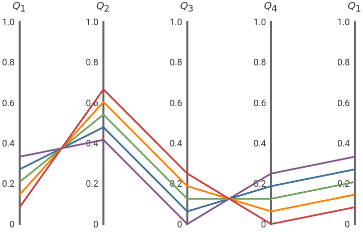
This Figure already illustrates the (anti-)correlation between the various . Correlation is further explored in Section 4.
Q
i
2
. Variational principles A possible resolution for an under-determined problem can be found by adopting a variational principle. This is a function of the joint probabilities to be optimized (maximized or minimized), while adhering to the constraints.
Sivia (p.112) proposes four different variational functions: entropy, sum of squares, sum of logarithms, sum of square roots, as shown in Table 5:
Table 5
In[]:=
Grid {"Variational principle",SpanFromLeft} ,{"","Function"} ,"Maximum entropy","- Log()" ,"Least squares"," " ,"Maximum logarithms"," Log()" ,"Maximum square roots"," " ,FrameAll ,ItemSize->{Automatic, 2}
n
∑
i=1
Q
i
Q
i
n
∑
i=1
2
Q
i
n
∑
i=1
Q
i
n
∑
i=1
Q
i
Out[]=
Variational principle | |
Function | |
Maximum entropy | - n ∑ i=1 Q i Q i |
Least squares | n ∑ i=1 2 Q i |
Maximum logarithms | n ∑ i=1 Q i |
Maximum square roots | n ∑ i=1 Q i |
The four variational functions are defined by
The four variational principle solution (VP) are found by minimizing or maximizing the above variational functions for the variable q1.
These four instantiations of the underdetermined problem are exploited in the paper in various roles. In this notebook, we will encounter many details associated with each of the four VP solutions.
Therefore, all results are combined in an Association[] named kangarooStructure[].
Therefore, all results are combined in an Association[] named kangarooStructure[].
Note that the MaxEnt and the LeastSq solutions are exact, whereas for MaxLog and MaxSqrt only a numerical approximation is available.
The Keys represent the variational principles:
The Values for the Keys are another Association[], and therefore kangarooStructure[] is a Nested Association. The inner Associations[] (Level 2) all have the same Key-Value structure. The MinMax key returns the extremal values of the VP solutions, for example the maximum of the entropy
or the minimum of the sum of squares
Results
Results
Table 6 and Figure 3 show the four solutions
Table 6
Figure 3
What does correlation and covariance actually mean? And what is the difference? Sometimes the two terms are even used interchangeably.
4.3 Covariance
4.3 Covariance
The variance-covariance matrix is defined by
Update Structure
Update Structure
The kangarooStructure[] is updated with the covariance matrix for all four principles:
4.4 Correlation
4.4 Correlation
The Correlation Coefficient is defined as
Therefore the correlation between the eye color and the dexterity of the kangaroos is
Update Structure
Update Structure
The kangarooStructure[] is updated with the correlation coefficient for all four principles:
4.5 Entropy
4.5 Entropy
The information entropy is defined as
We have defined the function entropyK[]
The entropy for the VP solutions is rescaled from nats to bits:
Update Structure
Update Structure
The kangarooStructure[] is updated with the information entropy for all four principles:
These quantities are all combined in Table 11:
Table 11
6.2 Tangent space
6.2 Tangent space
Figure 5
Figure 6
Figure 8
The ψ- coordinate system is restricted to the positive orthant:
Basis vectors
Basis vectors
The natural basis vectors of the tangent plane are defined by (Equation 56)
Perhaps, it would have been better to write
Update Structure
Update Structure
Store the basis vectors for all solutions with the Key “BasisVectors”:
Check
Vector angles
Vector angles
The basis vectors are not orthogonal
The basis vectors are also not normalized, their lengths are
However, they are perpendicular to the probability distribution
The angle ϕ is computed by VectorAngle[]: (Equation 59)
This is true for all four solutions
6.3 Metric tensor
6.3 Metric tensor
Figure 7
An extra FullSimplify[] makes it more readable:
The kangarooSymbolicMetricTensor is a symbolic expression which is used extensively in the upcoming computations. We also need a numerical version of this metric tensor, where the λ-s are replaced by numerical values:
The metric tensor for the LeastSq model solution (Equation 66)
and for the MaxEnt model (Equation 67)
6.4 Kullback-Leibler divergence
6.4 Kullback-Leibler divergence
Table 14
The KL-divergence table is not symmetric. Therefore, the KL divergence is not a proper distance.
6.6 Angular distances
6.6 Angular distances
Bhattacharyya angle
Bhattacharyya angle
We define a Bhattacharyya angle function:
Distance table
Distance table
With this result we can compute the distance table (in degrees) for our four Kangaroo models. This distance table is symmetric!
Table 15
Upper and lower limits
Upper and lower limits
In the text we make the assertion that (Equation 88)