Wolfram Cloud Document

Ref. 1 investigates the modeling and optimization of the gasification of wood chips. The model has been developed to correlate the gas composition (i.e. H2, CO), lower heating value (LHV), and cold gas efficiency (CGE) in terms of three independent variables : operation time, gas flow rate, and equivalence ratio. To do so, Response Surface Methodology (RSM) is used in conjunction with Box-Behnken design matrix. Our calculations using Mathematica agree closely with the results of Attri and Sharma. These later authors applied Design Expert software.

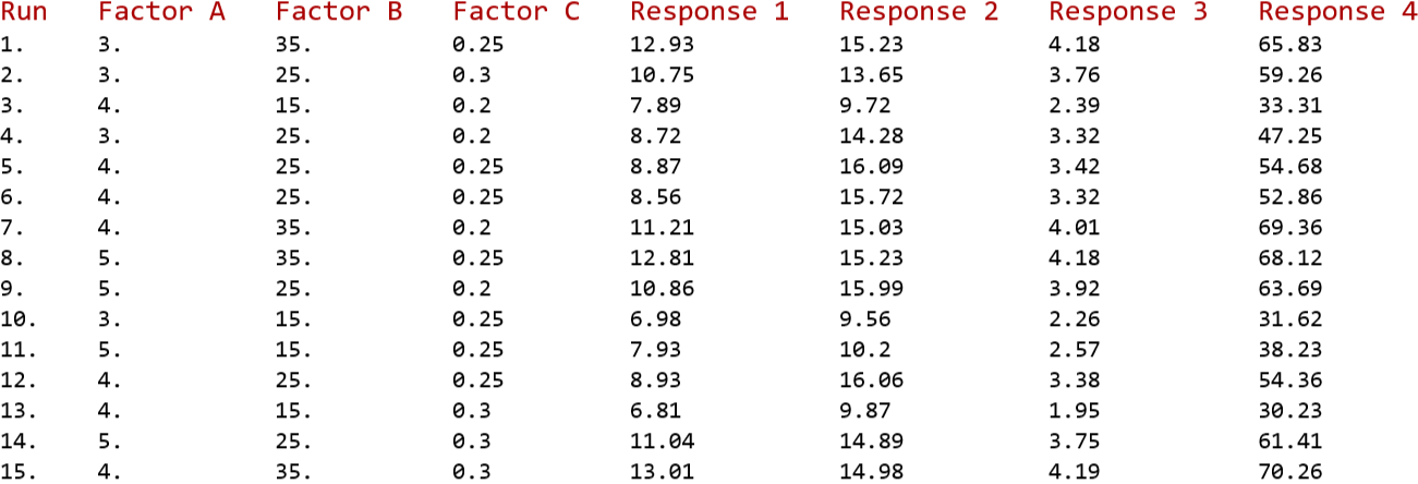
We assume the following responses for a Box-Behnken design matrix

In[]:=

data={{1.,3.,35.,0.25,12.93,15.23,4.18,65.83},{2.,3.,25.,0.30,10.75,13.65,3.76,59.26},{3.,4.,15.,0.20,7.89,9.72,2.39,33.31},{4.,3.,25.,0.20,8.72,14.28,3.32,47.25},{5.,4.,25.,0.25,8.87,16.09,3.42,54.68},{6.,4.,25.,0.25,8.56,15.72,3.32,52.86},{7.,4.,35.,0.20,11.21,15.03,4.01,69.36},{8.,5.,35.,0.25,12.81,15.23,4.18,68.12},{9.,5.,25.,0.20,10.86,15.99,3.92,63.69},{10.,3.,15.,0.25,6.98,9.56,2.26,31.62},{11.,5.,15.,0.25,7.93,10.2,2.57,38.23},{12.,4.,25.,0.25,8.93,16.06,3.38,54.36},{13.,4.,15.,0.30,6.81,9.87,1.95,30.23},{14.,5.,25.,0.30,11.04,14.89,3.75,61.41},{15.,4.,35.,0.30,13.01,14.98,4.19,70.26}};

Factors:
A : Gas flow rate (g/s), B : Operation time (minutes) andC : ER
Responses :
H2 (%) , CO (%) , LHV (MJ/kg) and CGE (%)

In[]:=

Join[{{Style["Run",Darker@Red,16],Style["Factor A",Darker@Red,16],Style["Factor B",Darker@Red,16],Style["Factor C",Darker@Red,16],Style["Response 1",Darker@Red,16],Style["Response 2",Darker@Red,16],Style["Response 3",Darker@Red,16],Style["Response 4",Darker@Red,16]}},data]//TableForm

Out[]//TableForm=

Range for factors are used to map coded to real values and vice versa

In[]:=

Mreal=Table[{data[[i]][[2]],data[[i]][[3]],data[[i]][[4]]},{i,1,15}]

Out[]=

{{3.,35.,0.25},{3.,25.,0.3},{4.,15.,0.2},{3.,25.,0.2},{4.,25.,0.25},{4.,25.,0.25},{4.,35.,0.2},{5.,35.,0.25},{5.,25.,0.2},{3.,15.,0.25},{5.,15.,0.25},{4.,25.,0.25},{4.,15.,0.3},{5.,25.,0.3},{4.,35.,0.3}}

In[]:=

Mreal//TableForm

Out[]//TableForm=

3.	35.	0.25
3.	25.	0.3
4.	15.	0.2
3.	25.	0.2
4.	25.	0.25
4.	25.	0.25
4.	35.	0.2
5.	35.	0.25
5.	25.	0.2
3.	15.	0.25
5.	15.	0.25
4.	25.	0.25
4.	15.	0.3
5.	25.	0.3
4.	35.	0.3

In[]:=

low={3,15,0.2};high={5,35,0.3};

In[]:=

mid=0.5(low+high)

Out[]=

{4.,25.,0.25}

In[]:=

halfrange=0.5(high-low)

Out[]=

{1.,10.,0.05}

coded values of the three factors

In[]:=

codedvar=Table[-(mid[[j]]-Mreal[[i,j]])/halfrange[[j]],{i,1,15},{j,1,3}]

Out[]=

{{-1.,1.,0.},{-1.,0.,1.},{0.,-1.,-1.},{-1.,0.,-1.},{0.,0.,0.},{0.,0.,0.},{0.,1.,-1.},{1.,1.,0.},{1.,0.,-1.},{-1.,-1.,0.},{1.,-1.,0.},{0.,0.,0.},{0.,-1.,1.},{1.,0.,1.},{0.,1.,1.}}

In[]:=

codedvar//TableForm

Out[]//TableForm=

-1.	1.	0.
-1.	0.	1.
0.	-1.	-1.
-1.	0.	-1.
0.	0.	0.
0.	0.	0.
0.	1.	-1.
1.	1.	0.
1.	0.	-1.
-1.	-1.	0.
1.	-1.	0.
0.	0.	0.
0.	-1.	1.
1.	0.	1.
0.	1.	1.

Visualize the design using Graphics3D

In[]:=

Show[Graphics3D[{Darker@Red,PointSize[0.025],Table[Point[codedvar[[i]]],{i,1,15}]}],Axes->True]

Out[]=

Forming MD the Computation Matrix

In[]:=

M=codedvar;

In[]:=

x1=Transpose[M][[1]]

Out[]=

{-1.,-1.,0.,-1.,0.,0.,0.,1.,1.,-1.,1.,0.,0.,1.,0.}

In[]:=

x2=Transpose[M][[2]]

Out[]=

{1.,0.,-1.,0.,0.,0.,1.,1.,0.,-1.,-1.,0.,-1.,0.,1.}

In[]:=

x3=Transpose[M][[3]]

Out[]=

{0.,1.,-1.,-1.,0.,0.,-1.,0.,-1.,0.,0.,0.,1.,1.,1.}

In[]:=

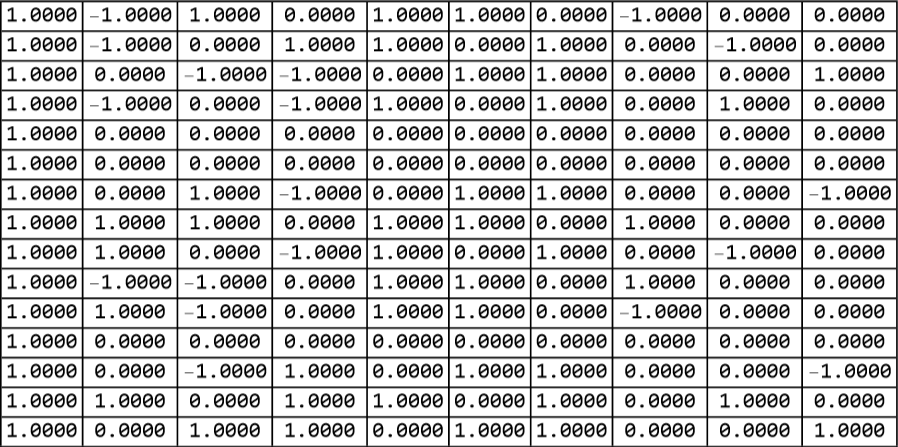
MD=Transpose[{{1.0000,1.0000,1.0000,1.0000,1.0000,1.0000,1.0000,1.0000,1.0000,1.0000,1.0000,1.0000,1.0000,1.0000,1.0000},x1,x2,x3,x1x1,x2x2,x3x3,x1x2,x1x3,x2x3}];

In[]:=

Grid[Table[NumberForm[MD[[i,j]],{4,4}],{i,1,15},{j,1,10}],Frame->All]

Out[]=

Using LinearModelFit to get the model for H2 in %

In[]:=

Clear[x1,x2,x3]

In[]:=

yexp=Table[data[[i]][[5]],{i,1,15}]

Out[]=

{12.93,10.75,7.89,8.72,8.87,8.56,11.21,12.81,10.86,6.98,7.93,8.93,6.81,11.04,13.01}

In[]:=

Dimensions[yexp]

Out[]=

{15}

In[]:=

datalm={MD,yexp}

Out[]=

{{{1.,-1.,1.,0.,1.,1.,0.,-1.,0.,0.},{1.,-1.,0.,1.,1.,0.,1.,0.,-1.,0.},{1.,0.,-1.,-1.,0.,1.,1.,0.,0.,1.},{1.,-1.,0.,-1.,1.,0.,1.,0.,1.,0.},{1.,0.,0.,0.,0.,0.,0.,0.,0.,0.},{1.,0.,0.,0.,0.,0.,0.,0.,0.,0.},{1.,0.,1.,-1.,0.,1.,1.,0.,0.,-1.},{1.,1.,1.,0.,1.,1.,0.,1.,0.,0.},{1.,1.,0.,-1.,1.,0.,1.,0.,-1.,0.},{1.,-1.,-1.,0.,1.,1.,0.,1.,0.,0.},{1.,1.,-1.,0.,1.,1.,0.,-1.,0.,0.},{1.,0.,0.,0.,0.,0.,0.,0.,0.,0.},{1.,0.,-1.,1.,0.,1.,1.,0.,0.,-1.},{1.,1.,0.,1.,1.,0.,1.,0.,1.,0.},{1.,0.,1.,1.,0.,1.,1.,0.,0.,1.}},{12.93,10.75,7.89,8.72,8.87,8.56,11.21,12.81,10.86,6.98,7.93,8.93,6.81,11.04,13.01}}

In[]:=

lm=LinearModelFit[datalm,{1,x1,x2,x3,x1x1,x2x2,x3x3,x1x2,x1x3,x2x3}]

Out[]=

FittedModel

8.79+0.408x1+8+0.366x3+0.562x3x3



In[]:=

Normal[lm]

Out[]=

8.78667+0.4075x1+0.994167x1x1-0.2675x1x2-0.4625x1x3+2.54375x2+0.381667x2x2+0.72x2x3+0.36625x3+0.561667x3x3

statistical and ANOVA analyses
A small p-value (typically < 0.05) means the variable significantly contributes to explaining the outcome.
A large p-value suggests the variable may not be important in the model and should be dropped from the model equation.

In[]:=

lm[{"ParameterTable","RSquared"}]

Out[]=



	Estimate	Standard Error	t-Statistic	P-Value
1	8.78667	0.243706	36.0543	3.0899× -7 10
x1	0.4075	0.149239	2.73052	0.0412548
x2	2.54375	0.149239	17.0448	0.0000127192
x3	0.36625	0.149239	2.45412	0.0576439
x1x1	0.994167	0.219674	4.52565	0.0062504
x2x2	0.381667	0.219674	1.73742	0.142818
x3x3	0.561667	0.219674	2.55682	0.0508427
x1x2	-0.2675	0.211056	-1.26744	0.260819
x1x3	-0.4625	0.211056	-2.19136	0.0799592
x2x3	0.72	0.211056	3.41142	0.0190141

,0.985875

Comparison of actual (exp .) and predicted values of response (H2 in %)

3-D and contour plot for x3=0

Using LinearModelFit to get the model for CO in %

Comparison of actual (exp .) and predicted values of response (CO in %)

3-D and contour plot for x3=0

Using LinearModelFit to get the model for LHV in MJ/kg

Comparison of actual (exp .) and predicted values of response (LHV in MJ/kg)

3-D and contour plot for x3=0

Using LinearModelFit to get the model for CGE in %

Comparison of actual (exp .) and predicted values of response (CGE in %)

3-D and contour plot for x3=0

References

◼

[1] Attri, V., Sharma, A.K. Modelling and optimization of gasification parameters of downdraft gasifier—an RSM approach. Biomass Conv. Bioref. 15, 5383–5400 (2025). https://doi.org/10.1007/s13399-024-05368-w

◼

[2] We also use the ideas for Placing a ContourPlot under a 3D Plot from: https://community.wolfram.com/groups/-/m/t/1148582

CITE THIS NOTEBOOK

Box-Behnken matrix for the modeling and optimization of biomass gasification
by Housam Binous, Asma Hammami, Hatem Dhaoudi and Ahmed Bellagi
Wolfram Community, STAFF PICKS, November 2, 2025
https://community.wolfram.com/groups/-/m/t/3569610

-1.	1.	0.
-1.	0.	1.
0.	-1.	-1.
-1.	0.	-1.
0.	0.	0.
0.	0.	0.
0.	1.	-1.
1.	1.	0.
1.	0.	-1.
-1.	-1.	0.
1.	-1.	0.
0.	0.	0.
0.	-1.	1.
1.	0.	1.
0.	1.	1.

-1.	1.	0.
-1.	0.	1.
0.	-1.	-1.
-1.	0.	-1.
0.	0.	0.
0.	0.	0.
0.	1.	-1.
1.	1.	0.
1.	0.	-1.
-1.	-1.	0.
1.	-1.	0.
0.	0.	0.
0.	-1.	1.
1.	0.	1.
0.	1.	1.

-1.	1.	0.
-1.	0.	1.
0.	-1.	-1.
-1.	0.	-1.
0.	0.	0.
0.	0.	0.
0.	1.	-1.
1.	1.	0.
1.	0.	-1.
-1.	-1.	0.
1.	-1.	0.
0.	0.	0.
0.	-1.	1.
1.	0.	1.
0.	1.	1.