Wolfram Cloud Document

Every river in mainland Great Britain, coloured by its catchment and line-weighted by Strahler order – the whole post in one picture. It is generated near the end with rnxFigRivers[gb, 1600, "Basin"]. The full 6667×11799 (78-megapixel) version is hosted in the Wolfram Cloud: open the high-resolution image.

Pour a bucket of water on a mountainside and it finds its way downhill, joining rivulets into streams and streams into rivers, until a single channel reaches the sea. The branching pattern it leaves behind is one of nature's most recognisable fractals – and the statistics of that branching are strikingly consistent from river to river. Big and small, wet and dry, drainage networks tend to fall in the same narrow range of scaling ratios, a regularity first noticed by Robert Horton in 1945 and sharpened by Arthur Strahler in 1952. How deep that regularity really runs – law of nature, or arithmetic of branching trees – is exactly what this post pokes at.

The setting. Our two rivers run almost side by side across Aberdeenshire, in the north-east shoulder of Scotland, and reach the North Sea barely three kilometres apart at the city of Aberdeen – whose very name marks the mouths (from the Pictish/Gaelic aber, a river mouth) of the Don and the Dee. Both rise high in the eastern Grampians: the River Dee at the Wells of Dee on the Braeriach plateau in the Cairngorms, around 1220 m up – one of the highest river sources in Britain – and the River Don near the Lecht a little to the north. The Dee then runs some 140 km east through Royal Deeside, past Balmoral (the Highland home Queen Victoria bought in 1852), and is one of the world's great Atlantic-salmon rivers; the Don, about 130 km long, powered the meal-mills and paper-works of old Aberdeenshire and is crossed near its mouth by the Brig o' Balgownie, a pointed Gothic arch begun under Robert the Bruce around 1320. Aberdeen itself, the Granite City, is literally built from the rock these rivers drain.

Why the land looks the way it does. The high ground is Cairngorm granite, a Caledonian pluton that crystallised roughly 400 million years ago and was later unroofed by erosion; the lower catchments are older Dalradian schists and gneisses. But the shape of the valleys is young. Through the Pleistocene ice ages the Cairngorms were a centre of glaciation, and ice gouged the corries, the deep troughs (Glen Dee, the Lairig Ghru) and the over-deepened valleys that today's rivers inherit. A regional eastward tilt sends almost everything to the North Sea – the very grain you will watch emerge from the elevation model. A drainage network is the slow bookkeeping of all this: every junction records where two flows, and two erosional histories, met.

This post does the whole thing from scratch in the Wolfram Language: download a real Digital Elevation Model, fill its pits, route the flow, accumulate drainage, extract the channel network, classify every stream by Strahler order, and test Horton's laws – for those two neighbouring catchments. The honest question is not just "do two rivers look alike?" but "how much can a handful of stream orders actually tell us?" So we will measure the ratios, put error bars on them, compare them to what pure chance would produce, and check how much they wobble when we change our arbitrary choices. The short answer: the number-law is robust, the rest is softer than the pretty pictures suggest, and that nuance is the interesting part.

All the heavy lifting lives in the companion package RiverNetworkX.wl – the only file you need beside this notebook. There are no data files to download separately and no API key: every cell is a one-liner whose call sits directly above its output. The outputs shown are pre-computed so the post opens instantly, but the notebook is fully self-contained – evaluate it and it fetches its own terrain from the built-in Wolfram GeoElevationData and recomputes everything from scratch (about a minute per river; a few more for all of Great Britain).

1. Setup

Load the package and build the two catchments. Each call downloads the terrain from the built-in GeoElevationData and runs the whole pipeline, returning an Association that carries the elevation grid, the flow-accumulation raster, the catchment mask, and the full Strahler-ordered stream graph. (The result is shown pre-computed; evaluate the cell to fetch and rebuild it live – about a minute each.)

SetDirectory[NotebookDirectory[]];Get["RiverNetworkX.wl"];(*eachcalldownloadsGeoElevationDataandextractsthenetwork–~1min,nokey*)dee=rnxBuildCatchment["Dee"];don=rnxBuildCatchment["Don"];

{dee["river"],Round[dee["areaKm2"]],don["river"],Round[don["areaKm2"]]}

{River Dee, 2167, River Don, 1825}

2. The elevation model

The terrain comes from the Wolfram Language's built-in GeoElevationData – no key, no download – which is what produced the walk-through here, at roughly 70 m resolution. A free OpenTopography key swaps in bare-earth EU_DTM 30 m instead, which (as section 10 shows) resolves finer channels; we use both and compare. The Dee rises high in the Cairngorms (the bright peaks in the west, near 1300 m) and runs east to Aberdeen; the Don drains the country just to the north.

ReliefPlotdee["grid"],



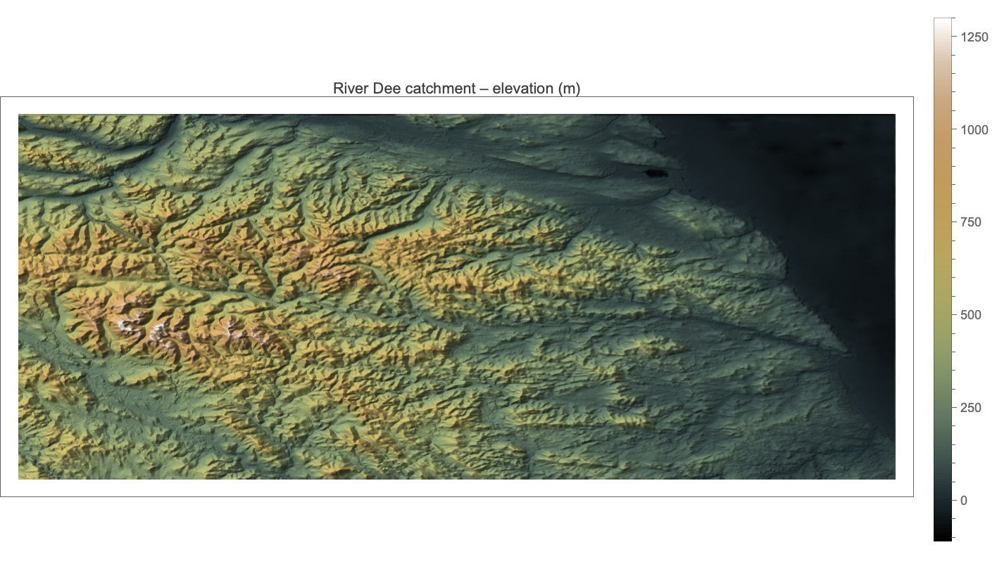
A DEM is nothing more than a raster of land-surface heights – here roughly one sample every 70–90 m, interpolated by GeoElevationData from public global terrain models (SRTM, ASTER, Copernicus and the like). Two things are worth knowing as data. First, it is a *surface* model: it records tree canopy and buildings as well as bare earth, which is why bare-earth products such as EU_DTM, which strip those off, route water through narrow valleys more faithfully – section 10 compares the two. Second, the grid is geographic (degrees of latitude and longitude), so a cell is not square on the ground; the package carries a per-row metric cell size (a degree of longitude shrinks as cos of latitude) so that lengths and areas come out in real metres. Read the relief above and you can already see the glacial fingerprint – the bright Cairngorm massif in the west, the troughs fanning eastward – before a single drop of water has been routed.

3. From elevation to flow: fill, direction, accumulate

Three classic steps turn a height field into a drainage network. First, depression filling (a Priority-Flood sweep) removes the spurious pits every DEM contains, so water can always escape to the sea. Second, D8 flow direction sends each cell's water to its steepest downhill neighbour, using true metric distances. Third, flow accumulation counts how many cells drain through each point – in a single O(n) pass, processing cells from high to low. The accumulation raster already looks like a river: the glowing dendritic tree below is just log₁₀ of the upstream cell count.

rnxFigDrainageArea[dee]

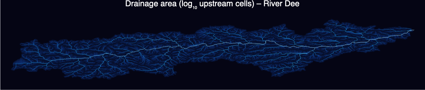
Channels emerge wherever accumulation exceeds a threshold (here a few hundred cells, ~5 km²). Everything upstream of the Aberdeen pour point is the catchment; its boundary is found by flooding the flow graph upstream from the outlet.

4. Stream order: the Strahler hierarchy

A century of stream ordering. The idea of ranking channels by hierarchy is Robert E. Horton's – an American hydraulic engineer often called the father of quantitative hydrology – in a landmark 1945 paper on the erosional development of drainage basins. Arthur N. Strahler, a geomorphologist at Columbia University, tidied Horton's scheme in 1952 into the topologically unambiguous form used here. Ronald Shreve added the complementary 'magnitude' (simply count the sources upstream) in 1966, and Eiji Tokunaga generalised the picture to side-branching in 1978. Between them, these few integers turn an unruly tangle of channels into something you can count, compare and fit.

Strahler's rule is beautifully simple. Every headwater stream is order 1. Where two streams of the same order ω meet, the result is promoted to order ω+1; where different orders meet, the larger simply continues. Order grows only when equals combine – exactly the logic in the package (ported from a Python reference: a junction promotes only when the two largest incoming orders are equal). Colouring each channel by its order reveals the skeleton of the basin: one thick trunk fed by an ever-finer hierarchy of tributaries.

rnxFigStrahlerNetwork[dee]

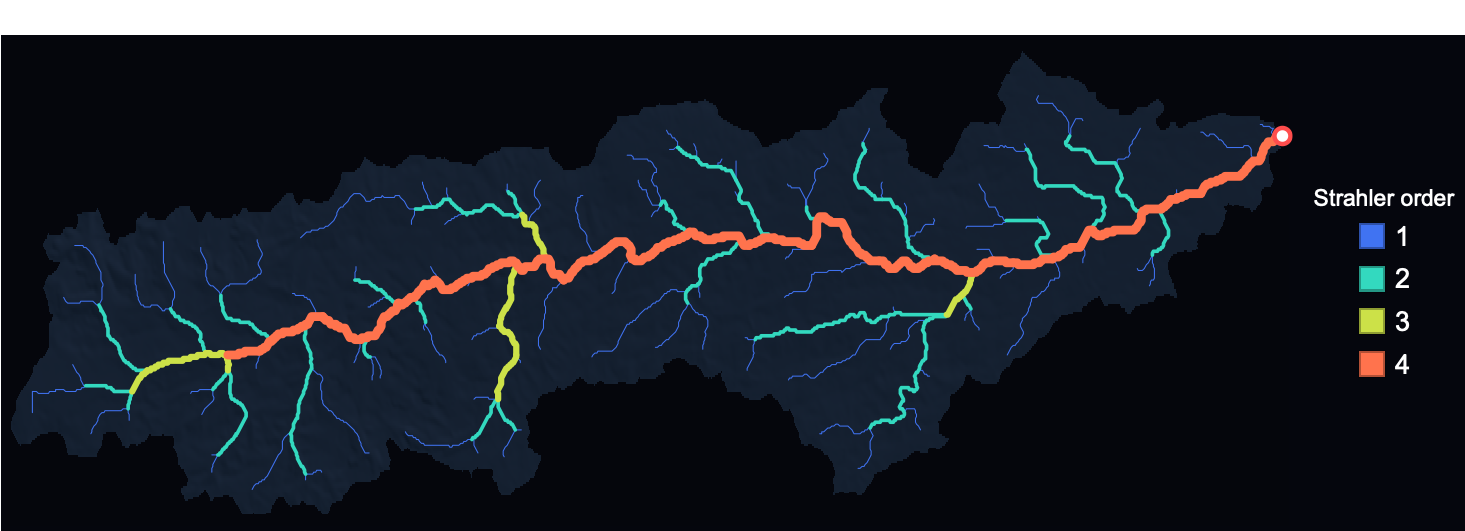
One subtlety that matters for getting the numbers right, and that trips up many home-grown implementations: a Strahler 'stream' of order ω is a *maximal chain* of connected order-ω links, not a single link. The Dee's order-4 trunk is one stream even though every tributary junction technically splits it into many links. Count links instead of streams and Horton's law of stream numbers breaks; count streams (as the package does) and it snaps straight.

5. The Dee and the Don, side by side

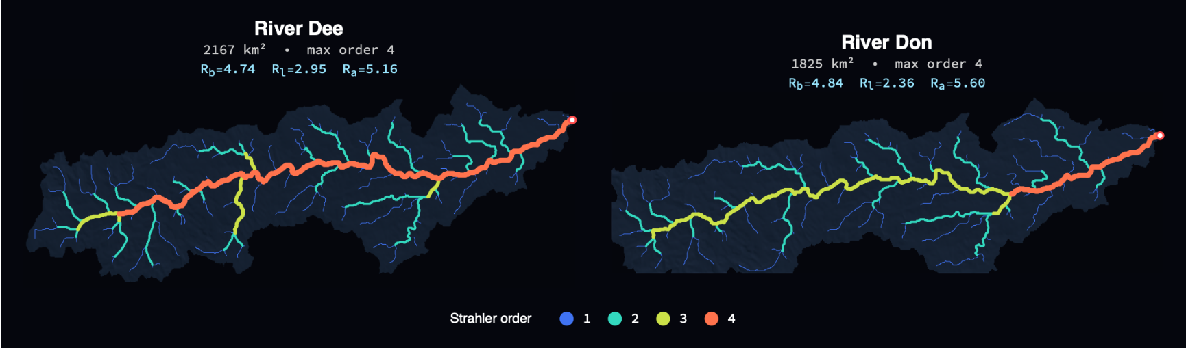
Two rivers, two independent extractions, on the same colour scale. They look like cousins, and the headline ratios under each come out close – though the error bars two sections from now will show that 'close' is doing a lot of work with only four orders to fit.

rnxFigCompareNetworks[dee,don]

6. Horton's laws

Horton's laws say that, climbing the order hierarchy, three quantities form geometric progressions:

◼

the number of streams of each order falls by a constant factor – the bifurcation ratio Rᵢ (typically 3–5);

◼

their mean length grows by the length ratio Rₗ (typically 1.5–3.5);

◼

their mean drainage area grows by the area ratio Rₐ (typically 3–6).

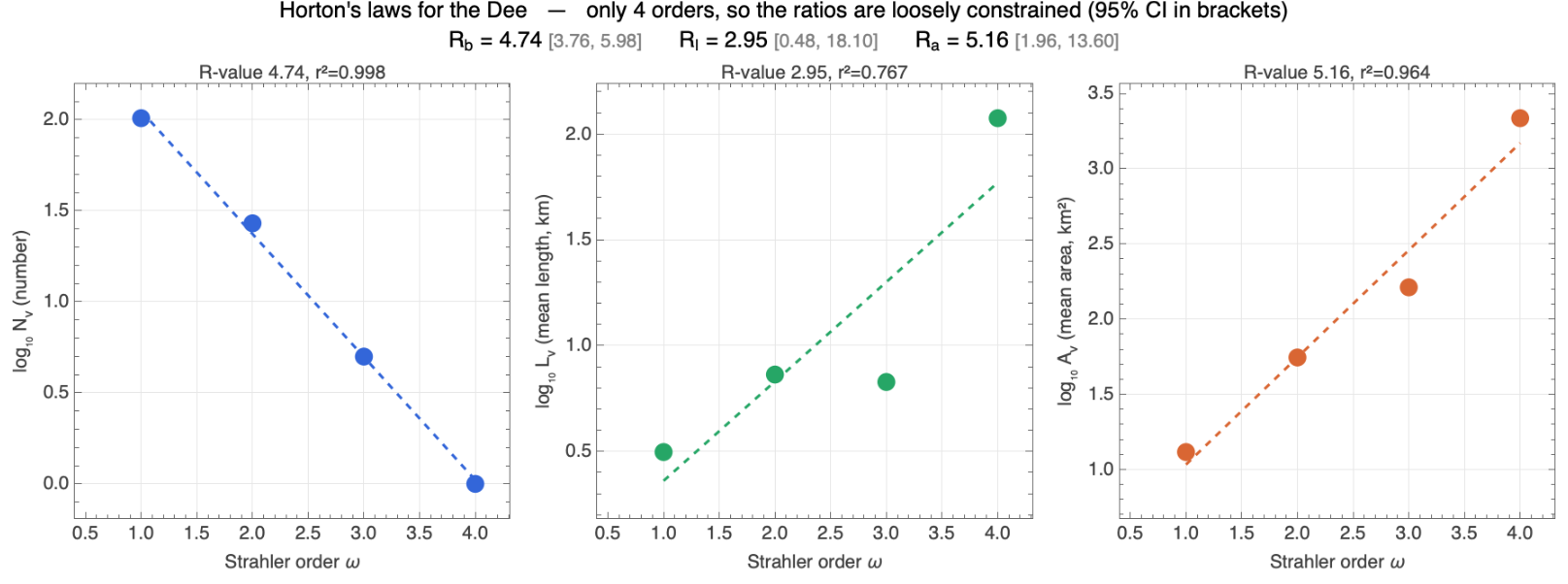
Equivalently, each quantity plotted on a log axis against integer order should fall on a straight line whose slope is the ratio. The raw numbers for the Dee:

rnxHortonRatios[dee["graph"]]//KeyTake[{"streamCounts","nOrders","Rb","Rb_CI","Rl","Rl_CI","Ra","Ra_CI"}]//Dataset

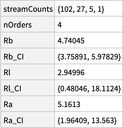
And the three laws as regression panels. The stream-number law is a near-perfect straight line; the area law is good; the length law is the ragged one. Crucially, with only four orders the slopes are loosely determined – so each panel carries a 95% confidence interval on its ratio, and those intervals are wide. The bifurcation ratio is pinned down (Rᵢ = 4.74, CI 3.8–6.0); the length ratio is barely constrained at all (Rₗ = 2.95, CI 0.5–18). Read the brackets, not just the point estimates.

rnxFigHortonLawPanels[dee]

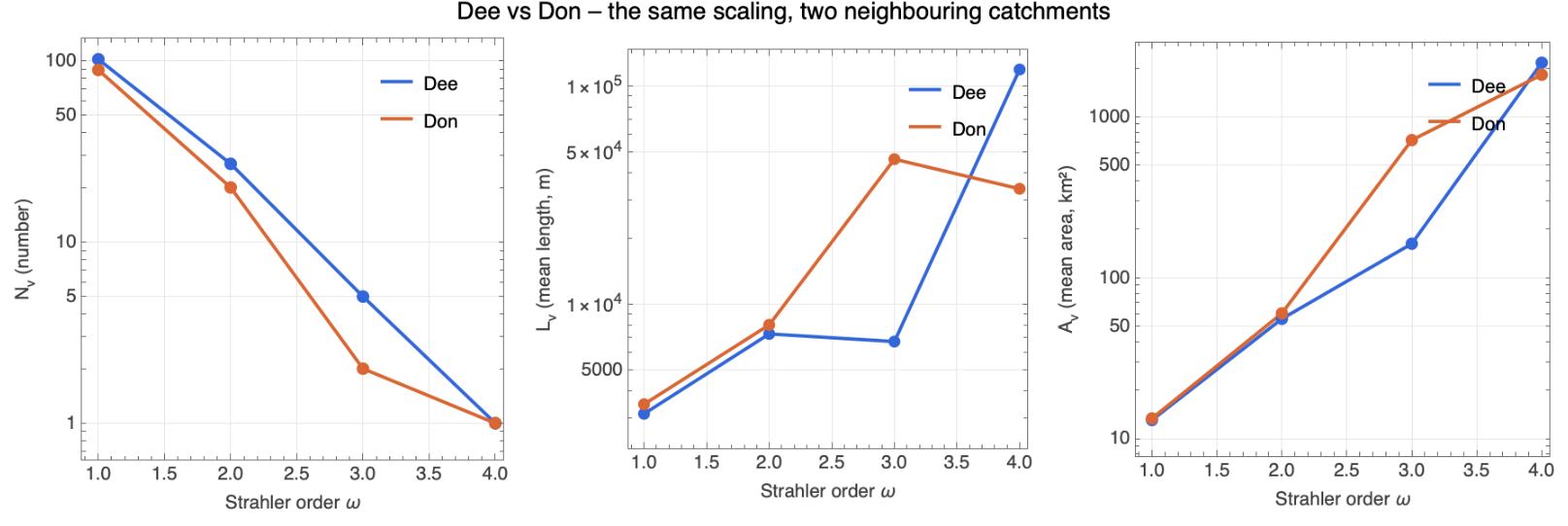
The same three panels for both rivers at once. The two catchments fall close together – visually compelling, and worth a second look at how much we should trust it (we do exactly that two sections on).

rnxFigHortonCompare[dee,don]

Side by side, the headline statistics:

The data-science health-warning, because it matters. Fitting a line to four points in log space and reading off a ratio is seductive, and Horton's laws almost always 'work' – which is precisely the catch. So let us actually test it. Take a random binary tree with the same number of headwater sources as the Dee (106) and grow it by merging branches at random, with no geomorphology at all; then measure its bifurcation ratio. Do that a few thousand times and you get a distribution:

Two lessons. First, pure randomness already produces a clean Horton hierarchy with Rᵢ ≈ 3 – geometric stream-number scaling is largely a property of branching trees, not a fingerprint of erosion (this is the point of Shreve 1966 and Kirchner's 1993 'Statistical inevitability of Horton's laws'). Different random ensembles land anywhere in Rᵢ ≈ 3–4.5, and real rivers in 4–5. Second, the Dee at 4.74 does sit a little above this particular null, so it is not merely random – there is some real structure. The honest reading: a matching Rᵢ between two rivers is necessary but weak evidence of a shared mechanism, because the whole family of branching networks lives in the same narrow band.

The other soft spot is the channel-initiation threshold – the accumulation at which we declare a channel to begin. It is genuinely arbitrary, and it controls everything downstream. Sweeping it across two orders of magnitude (here for Great Britain, re-using the cached flow) shows what is robust and what is not:

ukDEM = rnxLoadDEM[rnxCatchmentSpec["GreatBritain"]["bbox"], 8]; (* GeoElevationData *)
scan = rnxThresholdScanFromDEM[ukDEM, {20, 40, 70, 140, 280, 560, 1120, 2240}];
rnxFigThreshold[scan, ukDEM["meanCellArea"]/10.^6]

The drainage density and the maximum Strahler order depend strongly on the threshold (more sensitive channels → more orders, denser network), as does the length ratio Rₗ, which drifts by a factor of two. But the bifurcation ratio Rᵢ is reassuringly stable, hovering near 5 regardless. So of the three Horton ratios, only Rᵢ is both well-constrained and threshold-robust; Rₗ and Rₐ should be read with caution. That is the honest bottom line of this section.

7. Self-similarity: the Tokunaga picture

Horton's laws are a consequence of a deeper self-similarity. Tokunaga's description counts how many order-i tributaries attach to a typical order-j stream; for a self-similar tree this depends only on k = j−i and grows geometrically, Tₖ = a·c^(k−1). The fitted c here is close to the bifurcation ratio, as theory predicts.

8. The basin in three dimensions

Draping the order-coloured network over the terrain shows where the hierarchy lives: the trunk threads the valley floor while the fine tributaries climb the Cairngorm slopes. The output below is a live Graphics3D – drag to rotate, scroll to zoom. (It is embedded at a reduced mesh to keep the file small; re-evaluate the cell for the full-resolution surface.)

9. Three more signatures: Hack, width, hypsometry

Hack's law (1957) is the other great empirical scaling: the length of the longest channel grows as a power of drainage area, L ∝ A^h, classically with h ≈ 0.57. Over our nested sub-basins it is a clean power law (r² ≈ 0.96), with an exponent near 0.79 – steeper than the textbook 0.57. The Dee is a genuinely elongated basin – one long west–east trunk running from the Cairngorm plateau to the coast – and elongated basins make the longest channel grow almost in step with drainage area, which is exactly what a high Hack exponent records.

The width function counts how many channels lie at each distance from the outlet – a one-dimensional fingerprint of basin shape and a key control on the flood hydrograph.

And the hypsometric curves compare how area is distributed with elevation. Both basins have a hypsometric integral near 0.31 – well below 0.5, the signature of an old, deeply eroded landscape, exactly what you expect of the worn-down Grampians.

10. What we can and can't claim

What stands up: both rivers have a bifurcation ratio near 4.7 – well-constrained, threshold-robust, and squarely in the classic Horton range. Their drainage networks are genuinely self-similar (the Tokunaga and Hack fits are clean), and the basins are old and eroded (hypsometric integral ~0.31). At country scale the same Rᵢ ≈ 5 reappears across all of Britain. The bifurcation ratio is the one number here you can take to the bank.

What we should not oversell: the length and area ratios carry confidence intervals so wide (Rₗ = 2.95, CI 0.5–18) that 'the Dee and the Don agree' really means 'both are consistent with almost anything'; and because random branching trees already reproduce Horton-like scaling, matching ratios is weak evidence of a shared erosional mechanism. The fractal dimension D = log Rᵢ / log Rₗ inherits the length ratio's huge uncertainty, so we don't quote a single value.

Two DEMs, one basin. How much does the elevation source matter? Our no-key GeoElevationData is a ~70 m *surface* model; a free OpenTopography key swaps in bare-earth EU_DTM at 30 m (the Continental-Europe terrain model of Hengl et al., which strips vegetation and buildings). Running the identical pipeline on each is an independent check – and they agree on what matters most, the basin itself. The surface DEM puts the Dee at 2,167 km² and the bare-earth DEM at 2,093 km², both within a few percent of the gauged ~2,100 km². (Getting the area right hinges on one quiet detail: GeoElevationData returns each grid snapped outward to its tile pyramid, so the package recovers the true bounds before measuring – otherwise the cells, and the area, come out too small. The companion notebook overlays the computed network on the real OpenStreetMap rivers as an independent confirmation that it sits in the right place.) Where the two DEMs genuinely differ is resolution:

At 30 m the bare-earth model resolves finer tributaries and reaches a fifth Strahler order where the ~70 m surface model reaches four. Area tells a subtler story for the Don: bare-earth gives 1,321 km² (gauged 1,330), while the coarse surface extraction over-reaches a little into a neighbouring catchment (~1,830 km²) – resolution helps the routing as well as the detail. Both rivers, both DEMs, to order 5 on bare earth:

And here is the reassuring part for everything claimed above. Switching to an independent DEM at more than double the resolution barely moves the bifurcation ratio: Rᵢ goes 4.74 → 4.34 for the Dee and 4.84 → 4.00 for the Don, still squarely in the Horton band. The length and area ratios shift more (the Dee's Rₗ 2.95 → 2.42, Rₐ 5.16 → 4.44) – exactly as their wide confidence intervals warned. The one robust number stays put across both data sources; the soft ones stay soft.

The bigger picture. River networks were among Benoit Mandelbrot's original fractals; his celebrated 1967 question 'How long is the coast of Britain?' is a close cousin of the self-similarity we just measured – and, fittingly, Britain is the very coastline he asked about. The modern synthesis is Rodriguez-Iturbe and Rinaldo's 'Fractal River Basins: Chance and Self-Organization' (1997), which ties Horton's laws, Hack's law (mainstream length scaling with drainage area, L ~ A^0.57), and Tokunaga self-similarity to Optimal Channel Networks – configurations that minimise total energy dissipation and self-organise into the dendritic trees we see. The exponents are not arbitrary: they sit near the values an eroding landscape, forever balancing water, sediment and gravity, tends to find. That is the deeper reason the Dee, the Don and the whole of Britain rhyme.

11. Postscript: the whole of Great Britain

If the Dee and the Don obey the same law, how far does it go? Here is every river in mainland Great Britain, extracted the same way from a single ~500 m DEM (2.9 million cells). At a country scale the single-catchment pipeline becomes a FOREST – each river that reaches the sea is its own tree – and we keep only the largest land mass, so Ireland and the offshore islands drop out automatically. It is heavier (the depression-fill alone takes a few minutes), but it is still one self-contained call – the notebook downloads the country-wide terrain and extracts the whole forest itself:

The drainage-area map alone is a portrait of the country – the Tay and Spey draining the Highlands, the Severn and Thames in the south, the Pennine fan feeding the Trent and Ouse:

Coloured by Strahler order, the hierarchy lights up. The network reaches order 6 – the Tay, Spey, Severn, Thames and Trent are the thick warm trunks – fed by 3763 first-order headwaters:

And here is the call behind the image that opens this post – the same network in the style Robert Szucs made famous (Grasshopper Geography), every river coloured by the catchment it belongs to with line weight set by Strahler order. The downscaled version is the hook at the top of the post; evaluate the cell to render it yourself, or open the full 78-megapixel version in the Wolfram Cloud:

Full-resolution image: https://www.wolframcloud.com/obj/m.thiel/uk_rivers_GreatBritain_rainbow_hires.png

We can also colour the land itself by where its water goes. Labelling every cell with the sea-mouth it ultimately drains to partitions the whole country into its drainage basins – every translucent patch below is one catchment, washed in a cool synthwave palette over the dark relief (a golden-ratio hue hash keeps neighbours distinct), with each basin's river network glowing inside it in electric cyan, brightening with Strahler order so the trunks blaze and the headwaters shimmer. The big rivers become big patches threaded by a luminous main stem: the Trent–Ouse system draining to the Humber and the Wash dominates eastern England, the Tay and Spey take the Highlands, while the western coasts dissolve into a fine mosaic of short, steep catchments. These patches are exactly the basins whose internal statistics we have been measuring, now tiled across an entire island – mainland Britain partitions into about 20,000 of them, with nothing left over.

And Horton's laws, aggregated over every river in Britain. The number law is excellent across six orders (r² = 0.997) with a bifurcation ratio of 4.69 – the same value, again, as the Dee and the Don – and the area law is clean too (Rₐ = 3.40, r² = 0.99). The length law fails outright at this scale (r² ≈ 0.45): aggregating thousands of small steep catchments with a few large lowland ones is not a fair pooling, so there is no meaningful length ratio or fractal dimension here. The honest summary: the bifurcation ratio is remarkably stable from one glen to a whole island – which, given that random trees do much the same, says more about the arithmetic of branching than about British geology.

12. Reproduce it, and run it on your own river

There is nothing to reproduce separately – this notebook is the computation. Re-evaluate it and it downloads its own elevation data (Wolfram GeoElevationData) and rebuilds every figure. The whole pipeline for one catchment is a single call:

c = rnxBuildCatchment["Dee"]; (* download + fill -> ... -> Horton, ~1 min *)
rnxHortonRatios[c["graph"]]

For bare-earth EU_DTM 30 m instead of the ~70 m surface model – the upgrade that resolves finer detail and a fifth Strahler order in section 10 – register for a free OpenTopography key (no payment) and pass it as a second argument:

rnxBuildCatchment["Dee", "<your-free-OpenTopography-key>"] (* -> 2093 km², order 5 *)

And to map any river anywhere, point the public building blocks at your own bounding box and outlet – rnxLoadDEM, rnxFillSinks, rnxFlowDirectionD8, rnxFlowAccumulation, rnxDelineateCatchment, rnxNetworkGraph, rnxStrahlerOrder, rnxStreams, rnxHortonRatios, rnxTokunaga:

dem = rnxLoadDEM[{{56.80, 57.20}, {-3.90, -2.04}}, 10]; (* {{latS,latN},{lonW,lonE}} *)
c = rnxExtractNetwork[dem, {57.139, -2.075}, 400]; (* outlet lat/lon, threshold *)
rnxFigStrahlerNetwork[c]

CITE THIS NOTEBOOK

Every river in Britain: elevation drainage networks, Horton–Strahler statistics of the Dee & Don
by Marco Thiel
Wolfram Community, STAFF PICKS, June 4, 2026
https://community.wolfram.com/groups/-/m/t/3727475