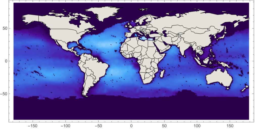
This example code illustrates how to access and visualize a NASA PO.DAAC AQUARIUS Level-3 Gridded HDF5 results file of Simulated Sea Surface Salinity
(*$TestPath="/Users/sdickson/Documents/test/HDF";SetDirectory[$TestPath];*)
Clear[]
In[]:=
$TestPath=FileNameJoin[{$HomeDirectory,"Documents","SPD_Viz","HDFEOS"}];
SetDirectory[NotebookDirectory[]];
AQUAfilename="Q20111212011151.L3m_MO_SCISM_V1.0_SSS_1deg.h5";
Import[AQUAfilename,"Elements"]
{Annotations,Data,DataEncoding,DataFormat,Datasets,Dimensions}
Transpose[{Import[AQUAfilename,"Datasets"],Import[AQUAfilename,"DataFormat"]}]
{{/l3m_data,Real32},{/palette,UnsignedInteger8}}
Import the dataset “/l3m_data”
l3mData=Import[AQUAfilename,{"Datasets","/l3m_data"}];
{latdim,londim}=Dimensions[l3mData]
{180,360}
Import[AQUAfilename,"Annotations"]
{{Scalinglinear,Scaling Equation(Slope*l3m_data) + Intercept = Parameter value,Slope1.,Intercept0.},{}}
From HDFView ATTRIBUTE ‘Parameter’
longName="Sea Surface Salinity";
From HDFView ATTRIBUTE ‘Units’
units="psu";
AbsoluteTiming[Histogram[l3mData]]
59.024045,
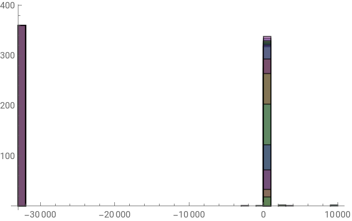
From HDFView: ATTRIBUTE ‘Data Minimum’ = -2488.2302
From HDFView: ATTRIBUTE ‘Data Maximum’ = 9765.761
From HDFView: ATTRIBUTE ‘Data Maximum’ = 9765.761
dataMin=Min[l3mData]
-32767.
fillValue=dataMin
-32767.
dataMax=Max[l3mData]
9765.76
From HDFView: ATTRIBUTE ‘Suggested Image Scaling Maximum’ = 38.0
From HDFView: ATTRIBUTE ‘Suggested Image Scaling Minimum’ = 32.0
From HDFView: ATTRIBUTE ‘Suggested Image Scaling Minimum’ = 32.0
The following works with Histogram[], but kills ListDensityPlot[]
dataFilled=ReplaceAll[l3mData,fillValueIndeterminate];
dataMin=Min[dataFilled]
Indeterminate
Histogram[dataFilled]
$Aborted
dataClipped=Clip[l3mData,{32.0,38.0}];
Needs["PlotLegends`"]
ShowLegend[ListDensityPlot[dataClipped,PlotRange{32.0,38.0},AspectRatio1/2,ColorFunction->"DeepSeaColors"],{ColorData["DeepSeaColors"][1-#1]&,10,"38.0","32.0",LegendPosition{1.0,-0.35},LegendLabelunits}]
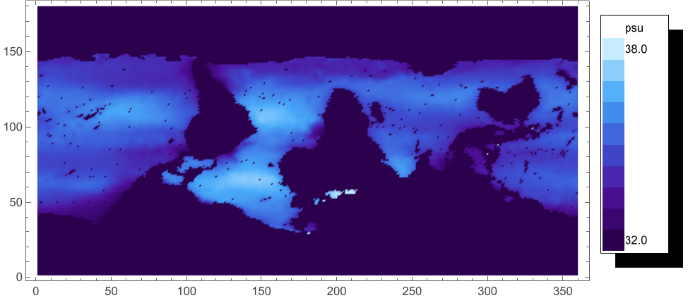
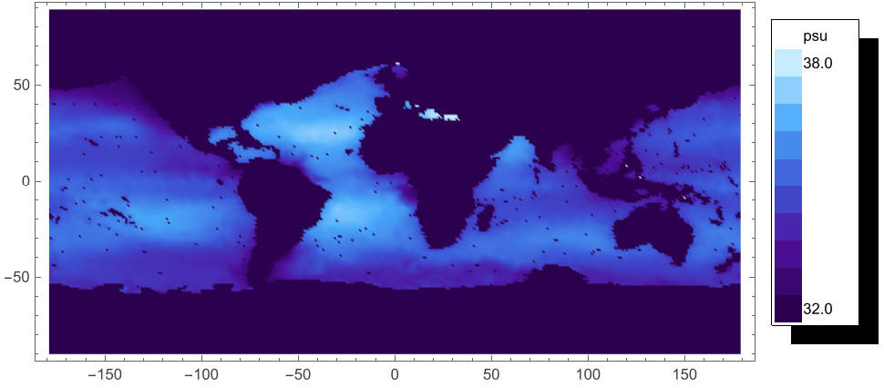
Assume that the Longitude/Latitude Grid Geolocation mapping is linear -- probably is for Geographic projection.
From HDFView: Easternmost Longitude = 180.0, Latitude Step = 1.0, Latitude Units = Degrees North, Longitude Step = 1.0,
Longitude Units = Degrees East, Map Projection = Equidistant Cylindrical, Northernmost Latitude = 90.0,
SW Point Latitude = -89.5, SW Point Longitude = -179.5, Southernmost Latitude = -90.0, Westernmost Longitude = -180.0
mapFun[lon_Integer,lat_Integer]:=Part[dataClipped,90-lat,180+lon]
latCoords=Table[90-(lat-1+0.5),{lat,-90,89},{lon,-180,179}];
Dimensions[latCoords]
{180,360}
lonCoords=Table[(lon-1+0.5)-180,{lat,-90,89},{lon,-180,179}];
Dimensions[lonCoords]
{180,360}
ShowLegend[ListDensityPlot[Flatten[Table[{lon,lat,mapFun[lon,lat]},{lon,-180,179,1},{lat,-90,89,1}],1],PlotRange{32.0,38.0},AspectRatio1/2,ColorFunction->"DeepSeaColors"],{ColorData["DeepSeaColors"][1-#1]&,10,"38.0","32.0",LegendPosition{1.0,-0.35},LegendLabelunits}]
ShowLegend[ListDensityPlot[Flatten[Table[{lon,lat,mapFun[lon,lat]},{lon,-180,179,1},{lat,-90,89,1}],1],PlotRange{32.0,38.0},AspectRatio1/2,ColorFunction->"DarkRainbow"],{ColorData["DarkRainbow"][1-#1]&,10,"38.0","32.0",LegendPosition{1.0,-0.35},LegendLabelunits}]
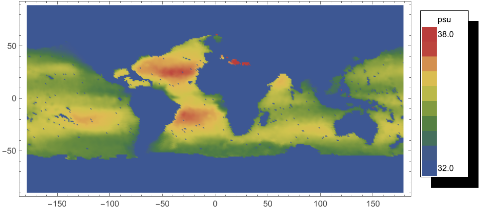
Show[{{ListDensityPlot[Flatten[Table[{lon,lat,mapFun[lon,lat]},{lon,-180,179,1},{lat,-90,89,1}],1],PlotRange{32.0,38.0},AspectRatio1/2,ColorFunction->"DeepSeaColors"],CountryData["World",{"Shape","Equirectangular"}]},Graphics[Legend[ColorData["DeepSeaColors"][1-#1]&,10,"38.0","32.0",LegendPosition{1.0,-0.35},LegendLabelunits]]}]