Problem
Problem
This question is posted for 2020 Team Selection Test/TST in Zhejiang Province for CMO.
In[]:=
<<MaTeX`
Out[]=

Analysis
Analysis
If you go directly use Maximize function, the answer is quite obvious
In[]:=
Maximize-,x>0,y>0,z>0,{x,y,z}
1
x+y+z+3
1
(x+1)(y+1)(z+1)
Out[]=
,{x2,y2,z2}
2
27
In[]:=
2
27
1
6
3
Out[]=
True
When it comes to explore the fine structure of this inequality, I find SliceContourPlot3D very helpful. If we take the LHS of the expression as function,
In[]:=
h[x_,y_,z_]:=-
1
x+y+z+3
1
(x+1)(y+1)(z+1)
h[x,y,z]
Say , thinking about mapping this unit cube to itself and assign a color to each point. This can be physically done with DensityPlot3D function. The option ClipPlanes is added to break the 3D body in half along the given plane.
{x,y,z}∈(0,1)x(0,1)x(0,1)
In[]:=
DensityPlot3D[h[x,y,z],{x,0.1,4},{y,0.1,4},{z,0.1,4},ClipPlanesInfinitePlane[{{0,0,0},{1,1,0},{1,1,1}}],OpacityFunctionScalingFalse,PlotLegendsAutomatic,ColorFunction"TemperatureMap",Boxed->False,AxesLabel{"x","y","z"},LabelStyle14]
Out[]=
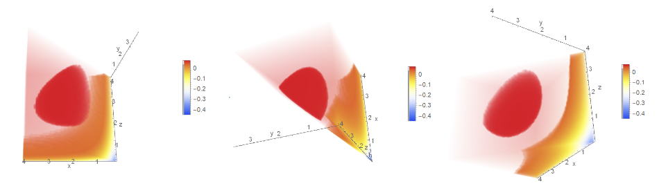
Base on the color distribution, the 3D plots give a rough idea but it is still quite hard to see the details. Directly working with this function may be far beyond the reach of high school students and the result may not be convincing unless some solid theoretic contents are discussed.
So I have to slice the spit cake. Given the cyclic symmetry of variables in the problem, it is wise to choose a control plane with constant sum of x, y and z. There are two ways to use this plot function
So I have to slice the spit cake. Given the cyclic symmetry of variables in the problem, it is wise to choose a control plane with constant sum of x, y and z. There are two ways to use this plot function
◼
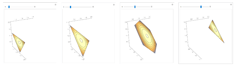
Scan the slicing plane so the contours and color functions are scaled on each plane locally. So it is pointless to compare the color across different planes.
Manipulate[SliceContourPlot3D[h[x,y,z],x+y+zη,{x,0.1,2},{y,0.1,2},{z,0.1,2},Contours10,BoxedFalse],{η,1,6}]
Out[]=
◼
Use DiagonalStackedPlanes as the second parameter of SliceContourPlot3D. Then the color is scaled across the values all slicing planes. Similarly, the number of contours specified is shared on all planes
In[]:=
SliceContourPlot3D-,{"DiagonalStackedPlanes",5},{x,0.1,4},{y,0.1,4},{z,0.1,4},Contours50,BoxedFalse
1
x+y+z+3
1
(x+1)(y+1)(z+1)
Out[]=

I prefer to use the first plot in this problem. The benefit is clear because is basically zero for large value of arguments. Thus the color distribution is flat in the second case. Also it shows there is a local maximum in each slice in the first plot. This can be proved clearly with the following argument with AM-GM over non negative values
h[x,y,z]
Out[]=

The equality sign is valid iff . Therefore we see the brightest color in the center of each contour plot. If we control , in which η is a constant. So is . At x = y = z = η/3,
x=y=z
x+y+z=η
1/η
◼
(x+1)(y+1)(z+1)
◼
1/ reaches minimum
(x+1)(y+1)(z+1)
which is equivalent to say -1/ reaches maximum. So does .
(x+1)(y+1)(z+1)
1/η-1/(x+1)(y+1)(z+1)
We can check the minimum quickly
In[]:=
SimplifyMinimize,0<x<η,0<y<η,x+y<η,{x,y},Assumptionsη>0
1
(x+1)(y+1)(η-x-y+1)
Out[]=
,xRoot4---+--#1++-&,1,yη-Root4---+--#1++-&,1
27
3
(3+η)
108
27+27η+9+
2
η
3
η
108η
27+27η+9+
2
η
3
η
27
2
η
27+27η+9+
2
η
3
η
54η
27+27η+9+
2
η
3
η
27
2
η
27+27η+9+
2
η
3
η
81
27+27η+9+
2
η
3
η
54η
27+27η+9+
2
η
3
η
2
#1
27
3
#1
27+27η+9+
2
η
3
η
1
2
108
27+27η+9+
2
η
3
η
108η
27+27η+9+
2
η
3
η
27
2
η
27+27η+9+
2
η
3
η
54η
27+27η+9+
2
η
3
η
27
2
η
27+27η+9+
2
η
3
η
81
27+27η+9+
2
η
3
η
54η
27+27η+9+
2
η
3
η
2
#1
27
3
#1
27+27η+9+
2
η
3
η
The root object looks scary but you can simplify it further by convert it to a rational function in terms of
t
In[]:=
Factor4---+--#1++-&[t]
108
27+27η+9+
2
η
3
η
108η
27+27η+9+
2
η
3
η
27
2
η
27+27η+9+
2
η
3
η
54η
27+27η+9+
2
η
3
η
27
2
η
27+27η+9+
2
η
3
η
81
27+27η+9+
2
η
3
η
54η
27+27η+9+
2
η
3
η
2
#1
27
3
#1
27+27η+9+
2
η
3
η
Out[]=
2
(-3t+η)
3
(3+η)
For non-negative η and t (also η >t because η is sum of three variable), the only way for the expression to be zero is t = η/3, which is the repeated root for x and y. Therefore the true maximum of the LHS of the original problem is
In[]:=
Maximize-,η,PositiveReals
1
η+3
27
3
(3+η)
Out[]=
,{η6}
2
27
which is same as picking the maximum of all maxima associated with η
Explore generalized cases
Explore generalized cases
Let’s look at the maximum value of the following expression with
k≥1
Out[]=

We may use the same argument as above. The key is to understand that the local maximum of each slicing plane is invariant w.r.t . For instance
k
k=2
In[]:=
Maximize-2*,η,PositiveReals
1
η+3
27
3
(3+η)
Out[]=
,η-3+9
-45+6(-3+9
2
)+2
(-3+9
2
)1458
2
2
In[]:=
Simplify[%]
Out[]=
,η-3+9
2
27
2
For any , we have
k≥1
In[]:=
SimplifyMaximize-k*,η,PositiveReals,Assumptionsk≥1
1
η+3
27
3
(3+η)
Out[]=
,ηRoot243--729k+162-#1+27--&,2
2
27
k
54
k
54
k
18
k
2
#1
2
3
#1
k
Factor the root object and we find the values all variables