Wolfram Computational Research Club at SUNY Korea
This essay investigates if foreign direct investment (FDI) helps economic growth more in middle-income countries. We use panel data from 2000 to 2024 for 100 countries. We use the Generalized Method of Moments (GMM) model with R.
1. Literature review
Past studies show FDI can help economic growth by bringing new capital and technology. But the effect is different for every country. Baiashvili & Gattini (2020) say that the effect of FDI on growth looks like an inverted-U shape based on a country’s income. This means middle-income countries get the most benefit from FDI. This essay uses the same idea but adds data up to 2024, which includes the COVID-19 period.
2. Research Questions and Hypotheses
The main question:
Does a country’s income level (GNI per capita) change how much FDI helps growth?
Hypothesis:
We expect FDI to help growth more as income rises, but only up to a point. After reaching upper-middle-income, the benefit likely starts to fall. This gives an inverted-U shape.
To test this, we add two extra terms to the model: FDI × log(GNIpc) and FDI × log(GNIpc)². If the coefficient on the squared term is negative and significant, it confirms the curve. Because FDI and growth can affect each other, we use Difference GMM with past growth as instruments, and we control for country and year differences.
3. Data sources and variables
Data source: World Bank
Time period: 2000–2024
Countries: 100 countries (25 per income group: Low, Lower-Middle, Upper-Middle, High Income), classified using World Bank GNI per capita. The 25 countries with the most complete data in the each group were selected.
Variables
GDPGrowth: Annual real GDP growth rate (Dependent)
FDI: Foreign Direct Investment net inflows (% of GDP)
GNIpc: GNI per capita (Income level)
FDI x log(GNIpc): Interaction term
FDI x log(GNIpc)²: An interaction term using the squared value of log(GNIpc).
Controls: GFCF, Government spending, Trade openness, Inflation
4. Data construction
1. Import, clean, and merge data
1. Import, clean, and merge data
We download seven CSV files from the World Bank, one for each variable. Each file has countries as rows and years as columns. We need to combine them into one dataset where each row is a country-year pair.
Import all World Bank CSVs from the working directory and reshape each into a long-format key-value table keyed by (CountryCode, Year):
In[]:=
SetDirectory[SystemDialogInput["Directory"]]
Out[]=
/Users/manaminomura/Downloads/Data
In[]:=
formatToLong[rawData_, varName_] := Module[{headerIdx, headers, years, rows}, headerIdx = SelectFirst[Range[Length[rawData]], MemberQ[rawData[[#]], "Country Code"] || MemberQ[rawData[[#]], "Country Name"] &]; If[MissingQ[headerIdx], headerIdx = 5]; headers = rawData[[headerIdx]]; rows = Drop[rawData, headerIdx]; years = Map[StringTake[ToString[#], 4] &, Drop[headers, 4]]; Association[Flatten[Table[val = row[[i + 4]]; numVal = Which[NumberQ[val], val, StringQ[val] && (val == "" || val == ".."), Missing[], StringQ[val], Quiet[ToExpression[StringReplace[val, "," -> ""]]], True, Missing[]]; If[NumberQ[numVal], {ToString[row[[2]]], years[[i]]} -> <|varName -> numVal|>, Nothing], {row, rows}, {i, Length[years]}]]]];csvFiles = FileNames["*.csv"];rawDatasets = Association @@ Table[FileBaseName[f] -> Import[f], {f, csvFiles}];vars = {"FDI", "GFCF", "GNIpc", "Government", "Growth", "Inflation", "Trade"};cleans = AssociationMap[formatToLong[rawDatasets[#], #] &, Select[vars, KeyExistsQ[rawDatasets, #] &]];mergedData = Merge[Values[cleans], Apply[Join]];finalRows = KeyValueMap[Join[{#1[[1]], #1[[2]]}, Values[#2]] &, mergedData];header = Join[{"CountryCode", "Year"}, Keys[First[mergedData]]];Export["data_for_gmm.csv", Prepend[finalRows, header]];
The result is saved as data_for_gmm.csv. Each row is one country in one year. Values shown as “..” in the original files are treated as missing and removed later in R.
4-2. Visualize FDI and GDP growth by income group
4-2. Visualize FDI and GDP growth by income group
Before running the model, we look at the raw data. We plot FDI against GDP growth for each income group. If the slope is steeper for middle-income countries than for high-income ones, that would support the inverted-U idea.
In[]:=
rPath = "/Library/Frameworks/R.framework/Resources/bin/Rscript";rCommand = "library(ggplot2)mydata <- read.csv('/Users/manaminomura/Downloads/Data/data_for_gmm_v3.csv', header = TRUE)colnames(mydata) <- gsub('[^[:alnum:]]', '', colnames(mydata))mydata <- subset(mydata, Year >= 2000)cols <- c('Growth', 'FDI', 'GNIpc')mydata[cols] <- lapply(mydata[cols], function(x) as.numeric(as.character(x)))mydata <- na.omit(mydata)mydata$Group <- cut(mydata$GNIpc, breaks = c(-Inf, 1085, 4255, 13205, Inf), labels = c('Low Income', 'Lower-Middle', 'Upper-Middle', 'High Income'))selected <- do.call(rbind, lapply(levels(mydata$Group), function(g) { sub <- subset(mydata, Group == g) yrs <- tapply(sub$Year, sub$CountryCode, length) chosen <- names(sort(yrs, decreasing = TRUE))[1:25] subset(sub, CountryCode %in% chosen)}))mydata <- selectedp <- ggplot(mydata, aes(x = FDI, y = Growth, color = Group)) + geom_point(alpha = 0.5, size = 1.5) + geom_smooth(method = 'lm', se = FALSE) + scale_color_brewer(palette = 'Set1') + xlim(-5, 20) + ylim(-10, 15) + labs(title = 'FDI vs Growth by Income Group (2000-2024)', x = 'FDI (% of GDP)', y = 'GDP Growth (annual %)', color = 'Income Group') + theme_minimal()ggsave('scatter_plot.png', p, width = 8, height = 6)";RunProcess[{rPath, "-e", rCommand}];Import["scatter_plot.png"]
Out[]=
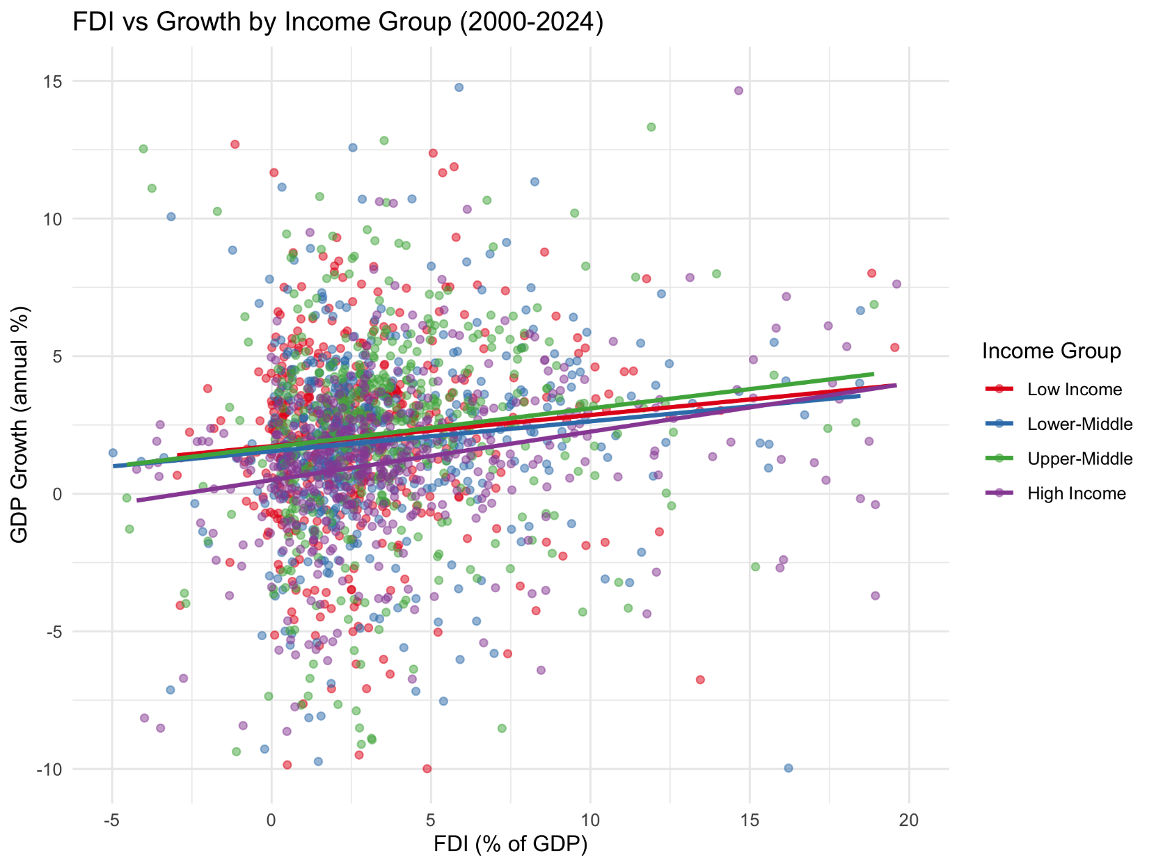
The plot shows that upper-middle-income countries have the steepest positive trend between FDI and growth. This pattern looks like an inverted-U, so we test it more carefully with the GMM model.
5. GMM model
5-1. Select 100 countries and run GMM model
5-1. Select 100 countries and run GMM model
We use the plm package in R to run a two-step Difference GMM model. The model includes last year’s growth (to account for persistence), FDI and its interaction terms, and four control variables. We control for both country and year effects, and use robust standard errors.
The key equation is
GDPGrowthᵢₜ = α·GDPGrowthᵢ,ₜ₋₁ + β₁·FDIᵢₜ + β₂·log(GNIpcᵢₜ) + β₃·FDIᵢₜ·log(GNIpcᵢₜ) + β₄·FDIᵢₜ·log(GNIpcᵢₜ)² + γ·Controlsᵢₜ + μᵢ + λₜ + εᵢₜ
If β₄ is negative and significant, it means FDI helps growth most at a middle income level and less after that — the inverted-U shape.
The key equation is
GDPGrowthᵢₜ = α·GDPGrowthᵢ,ₜ₋₁ + β₁·FDIᵢₜ + β₂·log(GNIpcᵢₜ) + β₃·FDIᵢₜ·log(GNIpcᵢₜ) + β₄·FDIᵢₜ·log(GNIpcᵢₜ)² + γ·Controlsᵢₜ + μᵢ + λₜ + εᵢₜ
If β₄ is negative and significant, it means FDI helps growth most at a middle income level and less after that — the inverted-U shape.
Classify countries into four income groups, select the 25 most data-complete countries per group, add log-income interaction terms, and run a two-step Difference GMM model with robust standard errors:
In[]:=
rPath = "/Library/Frameworks/R.framework/Resources/bin/Rscript";rCommand = "library(plm)mydata <- read.csv('/Users/manaminomura/Downloads/Data/data_for_gmm_v3.csv', header = TRUE)colnames(mydata) <- gsub('[^[:alnum:]]', '', colnames(mydata))mydata <- subset(mydata, Year >= 2000)cols <- c('Growth', 'FDI', 'GNIpc', 'GFCF', 'Government', 'Trade', 'Inflation')mydata[cols] <- lapply(mydata[cols], function(x) as.numeric(as.character(x)))mydata <- na.omit(mydata)mydata$Group <- cut(mydata$GNIpc, breaks = c(-Inf, 1085, 4255, 13205, Inf), labels = c('Low', 'Lower-Mid', 'Upper-Mid', 'High'))selected <- do.call(rbind, lapply(levels(mydata$Group), function(g) { sub <- subset(mydata, Group == g) yrs <- tapply(sub$Year, sub$CountryCode, length) chosen <- names(sort(yrs, decreasing = TRUE))[1:25] subset(sub, CountryCode %in% chosen)}))mydata <- selectedmydata$logGNI <- log(mydata$GNIpc)mydata$FDI_logGNI <- mydata$FDI * mydata$logGNImydata$FDI_logGNI_sq <- mydata$FDI * (mydata$logGNI^2)model <- pgmm( Growth ~ lag(Growth, 1) + FDI + logGNI + FDI_logGNI + FDI_logGNI_sq + GFCF + Government + Trade + Inflation | lag(Growth, 2:3) + lag(FDI, 2:2), data = mydata, index = c('CountryCode', 'Year'), effect = 'twoways', model = 'twosteps')print(summary(model, robust = TRUE))cat('\nCountries per group:\n')print(table(unique(mydata[, c('CountryCode','Group')])$Group))";result = RunProcess[{rPath, "-e", rCommand}];outputMessage = result["StandardOutput"] <> "\n" <> result["StandardError"];Print[Panel[outputMessage]]
The model passes the main diagnostic checks. The Sargan test suggests that the instruments are valid (p = 0.102). AR(1) is significant and AR(2) is not, which is the expected pattern for a valid Difference GMM model. In addition, the Wald test is highly significant (p < 0.001), showing that the model is jointly significant.
5-2. Plot marginal effect with 95% confidence interval
5-2. Plot marginal effect with 95% confidence interval
How much FDI helps growth changes with income level. We calculate this effect using the Delta Method:
dGrowth/dFDI = β₁ + β₃·log(GNIpc) + β₄·log(GNIpc)²
If the hypothesis is correct, the curve should go up from low income to middle income, then come down. A confidence interval above zero at middle income levels would confirm a real positive effect there.
dGrowth/dFDI = β₁ + β₃·log(GNIpc) + β₄·log(GNIpc)²
If the hypothesis is correct, the curve should go up from low income to middle income, then come down. A confidence interval above zero at middle income levels would confirm a real positive effect there.
Re-run the GMM model, compute the marginal effect of FDI at 200 equally-spaced income levels (log GNI 5 to 12), derive 95% confidence intervals via the Delta Method, and plot the result with income-group shading:
6. Results and Conclusion
The model was estimated using data from 100 countries between 2000 and 2024. The diagnostic tests support the model specification: the Sargan test does not reject instrument validity, AR(1) is significant, AR(2) is not, and the Wald test shows the model is significant.
Income level and trade openness have positive effects on growth, while government spending has a negative effect. The main hypothesis is not supported. Instead of an inverted-U relationship, the significant interaction terms suggest a U-shaped relationship between income level and the growth effect of FDI.
One possible explanation is that the COVID-19 period changed the normal relationship between FDI and growth. Another is that institutional quality, which is not included in the model, may influence how effectively countries benefit from FDI. Future research could test the robustness of these findings using additional institutional variables or System GMM estimation.
References
◼
Baiashvili, T., Gattini, L. (n.d.). Impact of FDI on economic growth: The role of country income levels and institutional strength. https://doi.org/10.2867/846546
◼
Croissant, Y., & Millo, G. (2008). Panel Data Econometrics inR: TheplmPackage. Journal of Statistical Software, 27(2). https://doi.org/10.18637/jss.v027.i02
◼
Millo, G. (2019). Estimating Robust Standard Errors for Financial Datasets with R and Plm: A Replication of Petersen’s Artificial Example, pp. 1–19, https://doi.org/10.13140/RG.2.2.16810.98247.
◼
Millo, G. (2017). Robust Standard Error Estimators for Panel Models: a Unifying Approach. Journal of Statistical Software, 82(3). https://doi.org/10.18637/jss.v082.i03
◼
R: Generalized Method of Moments (GMM) Estimation for Panel Data. (2026). R-Project.org. https://search.r-project.org/CRAN/refmans/plm/html/pgmm.html
◼
The World Bank. (2024). Foreign Direct investment, Net Inflows (% of GDP) | Data. Worldbank.org. https://data.worldbank.org/indicator/BX.KLT.DINV.WD.GD.ZS
◼
The World Bank. (2024). Gross fixed capital formation (% of GDP) | Data. Data.worldbank.org. https://data.worldbank.org/indicator/NE.GDI.FTOT.ZS
◼
The World Bank. (2024). GDP per capita growth (annual %) | Data. Worldbank.org. https://data.worldbank.org/indicator/NY.GDP.PCAP.KD.ZG
◼
The World Bank. (2024). General government final consumption expenditure (% of GDP) | Data. Data.worldbank.org. https://data.worldbank.org/indicator/NE.CON.GOVT.ZS
◼
The World Bank. (2024). GNI per capita, Atlas Method (current US$). Worldbank.org. https://data.worldbank.org/indicator/NY.GNP.PCAP.CD
◼
The World Bank. (2024). Inflation, consumer prices (annual %). Worldbank.org. https://data.worldbank.org/indicator/FP.CPI.TOTL.ZG
◼
The World Bank. (2024). Trade (% of GDP) | Data. Worldbank.org. https://data.worldbank.org/indicator/ne.trd.gnfs.zs
◼
Wickham, H. (2016). ggplot2: Elegant Graphics for Data Analysis. Springer. https://doi.org/10.1007/978-3-319-24277-4