ABSTRACT (original Article): An elastic map T associates stress with strain in some material. A symmetry of T is a rotation of the material that leaves T unchanged, and the symmetry group of T consists of all such rotations. The symmetry class of T describes the symmetry group but without the orientation information. With an eye toward geophysical applications, Browaeys & Chevrot developed a theory which, for any elastic map T and for each of six symmetry classes Σ, computes the “Σ-percentage” of T. The theory also finds a “hexagonal approximation”—an approximation to T whose symmetry class is at least transverse isotropic. We reexamine their theory and recommend that the Σ-percentages be abandoned. We also recommend that the hexagonal approximations to T be replaced with the closest transverse isotropic maps to T. CITATION (original Article): Tape, W., Tape, C. A Reformulation of the Browaeys and Chevrot Decomposition of Elastic Maps. J Elast (2024). https://doi.org/10.1007/s10659-024-10056-x
Our focus in this notebook is not specifically on the paper of Browaeys & Chevrot [1]. Rather, our goal is to provide enough code for you to analyze any elastic map and depict it as a contour plot on the unit sphere. In Section 1 we show how to construct the plot on the sphere. In Section 2, for any elastic map T and any elastic symmetry group , we show how to find the closest elastic map to T whose symmetry group includes . In Section 3, for any T and any symmetry class Σ, we show how to find a closest elastic map to T whose symmetry class is at least Σ. In Section 4 we show how to find the symmetry group of any T.
T
Selected references for this notebook are [2, 3, 4, 5, 8].
Some functions not specific to symmetry:
In[]:=
xyzTP[{θ_,ϕ_}]:={Cos[θ]Sin[ϕ],Sin[θ]Sin[ϕ],Cos[ϕ]};InnerProductMatrix[M_,N_]:=Flatten[M].Flatten[N];NormMatrix[M_]:=
;YRot[t_]:=
;ZRot[t_]:=
;id=IdentityMatrix[3];RandomRotation:=Module[{Uran},Uran=RandomVariate[CircularRealMatrixDistribution[3]];Det[Uran]Uran];Angle[u_,v_]:=ArcCos;
InnerProductMatrix[M,M]
;XRot[t_]:=1 | 0 | 0 |
0 | Cos[t] | -Sin[t] |
0 | Sin[t] | Cos[t] |
Cos[t] | 0 | Sin[t] |
0 | 1 | 0 |
-Sin[t] | 0 | Cos[t] |
Cos[t] | -Sin[t] | 0 |
Sin[t] | Cos[t] | 0 |
0 | 0 | 1 |
u.v
u.u
v.v
Some functions for formatting:
In[]:=
ScriptV[Σ_,U_]:=SequenceForm[SubscriptBox[Style["",13,Bold],Σ]//DisplayForm,"(",U,")"];ScriptT[Σ_]:=SubscriptBox[Style["",Bold],Σ]//DisplayForm;textβT[Σ_]:=SubsuperscriptBox["β ",Σ,"T"]//DisplayForm;textDT[Σ_]:=SubsuperscriptBox["d ",Σ,"T"]//DisplayForm;DegreeText[ξ_]:=Ifξ>=0,,-;MyRound[0.,k_]:=0;MyRound[x_,k_]:=Module{nn},nn=1;WhileRound[x-Floor[x],]0,IfFalse,Print"k = ",k,", nn = ",nn,", round = ",Roundx-Floor[x],;nn=nn+1;;NumberFormRoundx,,9;
"∘"
Round[ξ/Degree,.1]
"∘"
Round[Abs[ξ/Degree],.1]
-nn
10.
-(nn+k)
10.
-(nn-1+k)
10.
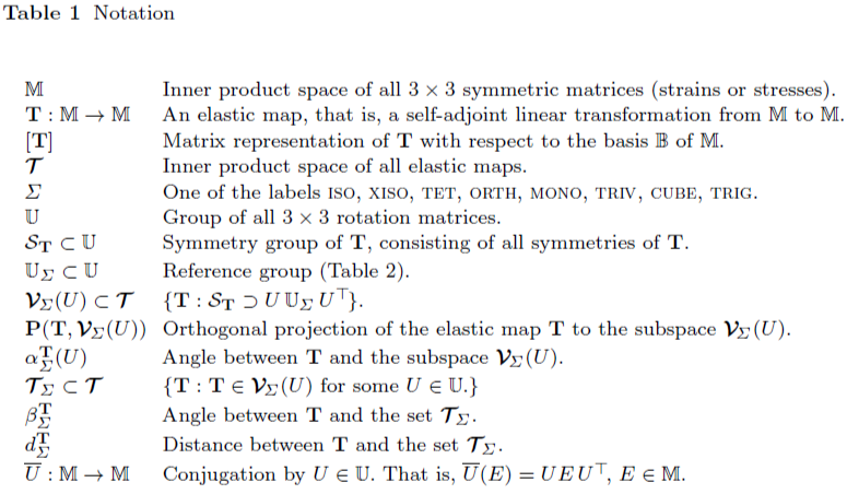
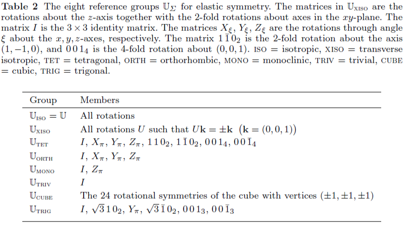
The eight reference matrices are given in Eq (81) of [8]. Their significance is explained in Eq (82).
Next is Eq (48) of [8], which defines the θσϕ coordinates for rotation matrices. The coordinates θ and ϕ are the spherical coordinates (longitude and colatitude) of the third column of the rotation matrix .
U
(θ,σ,ϕ)
In[]:=
UsHat[{θ_,σ_,ϕ_}]:=ZRot[θ].YRot[ϕ].ZRot[σ];
Section 1. Depicting an elastic map as a contour plot on the unit sphere.
Section 1. Depicting an elastic map as a contour plot on the unit sphere.
For us, matrix representations of a linear transformation are with respect to the orthonormal basis of . Its members are:
L:->
BB[1]=
; BB[2]=
; BB[3]=
;BB[4]=
; BB[5]=
; BB[6]=
;
0 | 0 | 0 |
0 | 0 | 1 2 |
0 | 1 2 | 0 |
0 | 0 | 1 2 |
0 | 0 | 0 |
1 2 | 0 | 0 |
0 | 1 2 | 0 |
1 2 | 0 | 0 |
0 | 0 | 0 |
- 1 2 | 0 | 0 |
0 | 1 2 | 0 |
0 | 0 | 0 |
1
6
1 | 0 | 0 |
0 | 1 | 0 |
0 | 0 | -2 |
1
3
1 | 0 | 0 |
0 | 1 | 0 |
0 | 0 | 1 |
Matrix representation [L] of L:
In[]:=
matrixL[L_]:=Table[InnerProductMatrix[L[BB[j]],BB[i]],{i,6},{j,6}];
This is the matrix of (Eq (32) of [8]):
U
In[]:=
MatrixUbar[U_]:=matrixL[U.#.Transpose[U]&]
Example of U and :
[]
U
In[]:=
Print["U = ",MatrixForm[ZRot[ξ]],", [] = ",MatrixForm[Simplify[MatrixUbar[ZRot[ξ]]]/.{-2Cos[ξ]Sin[ξ]->-Sin[2ξ]}]];
U
U =
, [] =
Cos[ξ] | -Sin[ξ] | 0 |
Sin[ξ] | Cos[ξ] | 0 |
0 | 0 | 1 |
U
Cos[ξ] | Sin[ξ] | 0 | 0 | 0 | 0 |
-Sin[ξ] | Cos[ξ] | 0 | 0 | 0 | 0 |
0 | 0 | Cos[2ξ] | -Sin[2ξ] | 0 | 0 |
0 | 0 | Sin[2ξ] | Cos[2ξ] | 0 | 0 |
0 | 0 | 0 | 0 | 1 | 0 |
0 | 0 | 0 | 0 | 0 | 1 |
The subspace (U) consists of the elastic maps that have as a 2 - fold point. The elastic map is the closest such map to T.
MONO
U
k
P(T,(U))
MONO
Next are Eqs (84e), (31a), (31b) of [8]. They give .
P(T,(U))
MONO
In[]:=
ProjToVSigOfU
,id,MONO:=
;ProjToVSigOfU[Tmat_,U_,Σ_]:=MatrixUbar[U].ProjToVSigOfU[Amat[Tmat,U],id,Σ].Transpose[MatrixUbar[U]];Amat[Tmat_,U_]:=Transpose[MatrixUbar[U]].Tmat.MatrixUbar[U];
a_ | g_ | m_ | q_ | t_ | v_ |
gdum_ | b_ | h_ | n_ | r_ | u_ |
mdum_ | hdum_ | c_ | i_ | o_ | s_ |
qdum_ | ndum_ | idum_ | d_ | j_ | p_ |
tdum_ | rdum_ | odum_ | jdum_ | e_ | k_ |
vdum_ | udum_ | sdum_ | pdum_ | kdum_ | f_ |
a | g | 0 | 0 | 0 | 0 |
g | b | 0 | 0 | 0 | 0 |
0 | 0 | c | i | o | s |
0 | 0 | i | d | j | p |
0 | 0 | o | j | e | k |
0 | 0 | s | p | k | f |
Example 1
Example 1
This is (the matrix of) the elastic map T in Sections 7 and 8 of [8]):
In[]:=
TmatExample1=
;MatrixNote[TmatExample1]="Tmat is TmatExample1";Print[MatrixNote[TmatExample1]];TmatExample1==Transpose[TmatExample1]
206.2 | -67.4 | 17.1 | -15.9 | 166.6 | -19.5 |
-67.4 | 352.9 | 32.2 | 3.3 | 61.6 | -41.6 |
17.1 | 32.2 | 343.8 | 0.4 | 73.6 | -4.2 |
-15.9 | 3.3 | 0.4 | 270. | 88.8 | 13.3 |
166.6 | 61.6 | 73.6 | 88.8 | 287.1 | 30.7 |
-19.5 | -41.6 | -4.2 | 13.3 | 30.7 | 74. |
Tmat is TmatExample1
Out[]=
True
In[]:=
Tmat=TmatExample1;
If you use an elastic map of your own, your matrix is apt to be a Voigt matrix and will need to be converted to a representation Tmat with respect to the basis . To go back and forth between Voigt and Tmat (Section S5.3 of [6]):
In[]:=
TmatOfVoigt[Voigt_]:=Simplify[IsubBΣ.Voigt.IsubΥB];VoigtOfTmat[Tmat_]:=Simplify[Inverse[IsubBΣ].Tmat.Inverse[IsubΥB]];IsubBΣ=
;IsubΥB=
;
0 | 0 | 0 | 2 | 0 | 0 |
0 | 0 | 0 | 0 | 2 | 0 |
0 | 0 | 0 | 0 | 0 | 2 |
- 1 2 | 1 2 | 0 | 0 | 0 | 0 |
1 6 | 1 6 | - 2 3 | 0 | 0 | 0 |
1 3 | 1 3 | 1 3 | 0 | 0 | 0 |
0 | 0 | 0 | - 1 2 | 1 6 | 1 3 |
0 | 0 | 0 | 1 2 | 1 6 | 1 3 |
0 | 0 | 0 | 0 | - 2 3 | 1 3 |
2 | 0 | 0 | 0 | 0 | 0 |
0 | 2 | 0 | 0 | 0 | 0 |
0 | 0 | 2 | 0 | 0 | 0 |
Example:
contours[Tmat, Σ, delN] and MaxForScaling[Tmat, Σ] give the option of having the same contours and color scheme for multiple elastic maps, so that the maps can be compared.
Example:
If desired, the above MaxForScaling can usually be decreased slightly to give redder colors at the high end:
Example of cpMONOprelim. The plot will take a minute or so.
The ambient lighting (second sphere) is less aesthetic but more informative.
Example 2
Example 2
This is the tetragonal map in Section 10.4 of [8].
We had to move the first small sphere outward to avoid overcrowding :
Eq . (16) of [8] is
Example of nminimize:
Rarely, NMinimize will fail. That is, it will find a local min that is not a global min. We therefore run it two or three times:
Some functions involving nminimize :
A Σ-minimizer for T (Eq (46) of [8 ]):
A closest elastic map to T having symmetry at least Σ:
Example :
The main goal of this section has thus been realized.
The command MinimizationFacts, below, summarizes some of the consequences.
The main goal of this section has thus been realized.
The command MinimizationFacts, below, summarizes some of the consequences.
The command MinimizationFacts, below, summarizes some of the consequences.
From Eq (12) of [8]:
MinimizationFacts is just for formatting output.
In this section we are implementing Theorem 3 of [7].
Code for ≺ :
DeriveSymGp may take a minute or so, since many minimizations are involved.
Choose a Tmat or make up your own:
Choose a Tmat or make up your own:
References
References
[1] Browaeys, J.T., Chevrot, S.: Decomposition of the elastic tensor and geophysical applications. Geophys. J. Int. 159, 667–678 (2004). https://doi.org/10.1111/j.1365-246X.2004.02415.x
[2] Joe Dellinger. Computing the optimal transversely isotropic approximation of a general elastic tensor. Geophysics, 70(5):i1–10, 2005.
[3] Çağri Diner, Mikhail Kochetov, and Michael A. Slawinski. On choosing effective symmetry classes for elasticity tensors. Q. J. Mech. Appl. Math., 64(1):57–4, 2010. https://doi.org/10.1093/qjmam/hbq023
[4] Sandra Forte and Maurizio Vianello. Symmetry classes for elasticity tensors. J. Elasticity, 43:81–108, 1996.
[5] M. François, G. Geymonat, and Y. Berthaud. Determination of the symmetries of an experimentally determined stiffness tensor: application to acoustic measurements. Int. J. Solids Structures, 35(31–32):4091–4106, 1998. https://doi.org/10.1016/S0020-7683(97)00303-X
[6] Tape, W., Tape, C.: Elastic symmetry with beachball pictures. Geophys. J. Int. 227, 970–1003 (2021). https://doi.org/10.1093/gji/ggab183
[7] Tape, W., Tape, C.: Two complementary methods of inferring elastic symmetry. J. Elast. 150, 91–118 (2022). https://doi.org/10.1007/s10659-022-09898-0
[8] Tape, W., Tape, C. A Reformulation of the Browaeys and Chevrot Decomposition of Elastic Maps. J Elast (2024). https://doi.org/10.1007/s10659-024-10056-x
CITE THIS NOTEBOOK
CITE THIS NOTEBOOK
A reformulation of the Browaeys and Chevrot decomposition of elastic maps
by Walter Tape & Carl Tape
Wolfram Community, STAFF PICKS, May 22, 2024
https://community.wolfram.com/groups/-/m/t/3180725
by Walter Tape & Carl Tape
Wolfram Community, STAFF PICKS, May 22, 2024
https://community.wolfram.com/groups/-/m/t/3180725