The main goal of this project is to explore dimensional decay in the evolution of densely connected hypergraphs. We give a systematic investigation of rules with signature . Shrinking of the mean vertex connectivity of the hypergraphs indicates a decay of Hausdorff dimension. We verify this numerically for a set of interesting rules. We classify possible hypergraph behaviours in four different categories. The most promising rules lead to dimensional decay followed by a plateau at the limit of large number of time steps. Moreover, this is qualitatively insensitive to the change inner connection configuration. Observed dimensional decay is relevant in the context of early universe cosmology as an alternative for inflation.
2
2
2
2
Initialization
Initialization
SetOptions[EvaluationNotebook[],DockedCellsNone]listEvolution[r_,InitialCondition_]:=NestWhileList[ResourceFunction["WolframModel"][r,#1,1,"FinalState"]&,InitialCondition,(!IsomorphicGraphQ[SimpleGraph@Graph[UndirectedEdge@@@#1],SimpleGraph@Graph[UndirectedEdge@@@#2]]&&ResourceFunction["ConnectedHypergraphQ"][#1])&,2,100]finalEvolution[r_,InitialCondition_]:=NestWhile[ResourceFunction["WolframModel"][r,#,1,"FinalState"]&,InitialCondition,(!IsomorphicGraphQ[SimpleGraph@Graph[UndirectedEdge@@@#1],SimpleGraph@Graph[UndirectedEdge@@@#2]]&&ResourceFunction["ConnectedHypergraphQ"][#2])&,2,100]listEvolution2[r_,InitialCondition_]:=NestWhileList[ResourceFunction["WolframModel"][r,#1,1,"FinalState"]&,InitialCondition,(!IsomorphicGraphQ[SimpleGraph@Graph[UndirectedEdge@@@#1],SimpleGraph@Graph[UndirectedEdge@@@#2]]&&ResourceFunction["ConnectedHypergraphQ"][#1])&,2,300]InitialConditionFullyConnected=Tuples[Range[10],2];RuleSet=ResourceFunction["EnumerateWolframModelRules"][{{2,2}}{{2,2}}];
Motivation
Motivation
On the large scales, observed universe is isotropic and homogeneous. This is clearly seen in the Cosmic Microwave Background Radiation, which is a “snapshot” of the last photon scattering on protons around 370,000 years after the Big Bang. Shortly before this time, the universe was filled with electrically charged plasma and the average free path of a photon was extremely short, the universe was non-transparent. While expanding, the universe cooled down to temperatures in which protons bound with electrons creating electrically neutral hydrogen. This is known as a process of recombination, after which photons propagated freely. Light from that time reaches earth (red-shifted to microwave lengths) with the spectrum characteristic of perfectly black body at temperature around 2.725 K. Remarkably, the temperature is the same, independent of the direction of observation! The temperature fluctuations are 5 orders of magnitude smaller than the globally observed value [1]. CMB Spectrum Blue regions correspond to lower temperature, while red regions to the higher temperature
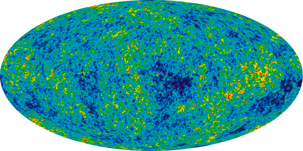
This fact was puzzling to cosmologists for years. CMB data implies that the temperature of the plasma universe before the recombination was almost the same everywhere. This is rather peculiar, since it means that the whole universe must have been in a thermal equilibrium, even though the speed of the heat transfer was bounded from above by the speed of light. There was no way (in the framework of Friedmann equations with the radiation dominated universe) for the universe to exchange heat fast enough to remain in the thermal equilibrium.
Cosmological inflation provides an elegant way of solving this riddle. It states that initially (or at least s after the Big Bang) the universe was pointlike, then it went trough an inflationary phase, growing exponentially more than times in just seconds. Such an incredible speed of inflation globally “preserved” the equilibrium. Cosmological inflation is now a well established theory in great agreement with the CMB data. It is responsible for creating large scale structures in the universe and gives a seed for quantum fluctuations present in the CMB.
-35
10
50
-33
10
In the context of Wolfram Model [2], we may model the initial, equilibrium state of the universe by considering densely connected hypergraphs. When a graph is densely connected it takes only few steps to reach any other vertex. This suggests that it will have large Hausdorff dimension. From the cosmological point of view it is interesting to see whether fully connected initial conditions lead to dimensional decay during the evolution of the hypergraph (spoiler, they do). High connectivity may also be understood as larger-than-normal speed of light, which should asymptotically converge to the measured value. Moreover, the dense connectivity corresponds to the increased causal connectivity similarly as in the theory of inflation.
Introduction
Introduction
As a model of the early, highly-dimensional universe we treat fully connected hypergraphs. This means that the effective distance between any two vertices is equal to 1. We explore rules with signature as the first step towards a more general result. Here is an example of the initial condition with 10 vertices.
2
2
2
2
Out[]=
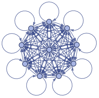
The rules we are considering will transform a pair of edges into another pair of edges, possibly adding new vertices. For example
RulePlot[ResourceFunction["WolframModel"][#],VertexLabelsAutomatic]&[{{1,2},{3,2}}{{1,4},{4,2}}]
Out[]=

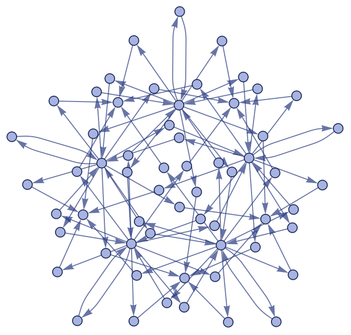
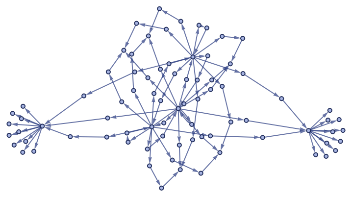
This results in a growing tree-like evolution of the hypergraph, which stops after 4 steps.
Out[]=
,
,
,
,
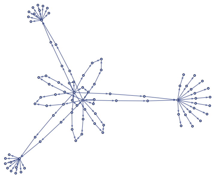
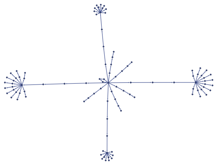
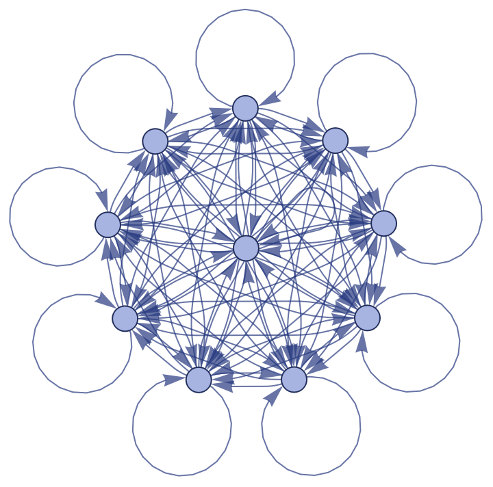
At first sight the average number of edges attached to a node shrinks. Shrinking of the mean vertex connectivity will indicate a decay of Hausdorff dimension. In the following section we will verify this numerically for a set of interesting rules.
There are in total 562 rules with signature and they lead to the four main classes of behaviour:
There are in total 562 rules with signature
2
2
2
2
1
.Inapplicable rule- in majority of cases a rule cannot be applied to the hypergraph shortly after the beginning of the evolution
2
.Hypergraph disconnection
3
.Isomorphic evolution- vertices of a hypergraph are merely relabeled during the evolution
4
.Periodic evolution- hypergraph oscillates between a few states (usually 2 or 3)
All of the investigated rules fall into one of these categories, so there are no systems evolving eternally. However, we have found a set of rules which stop after a considerable number of steps. Possible number of steps before halting is also dependent on the size of initial condition. Here we provide a set exemplary final states (we terminate the evolution once one of the conditions 1-3 is satisfied).
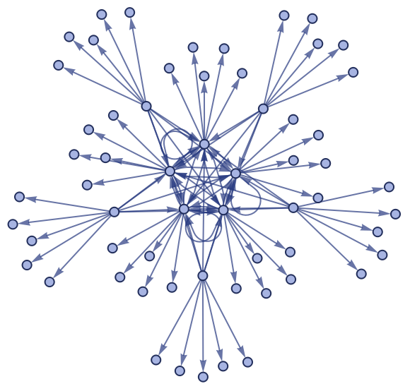
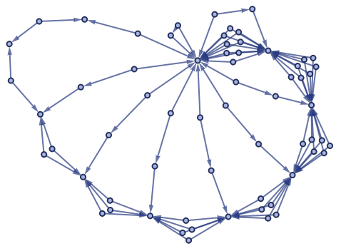
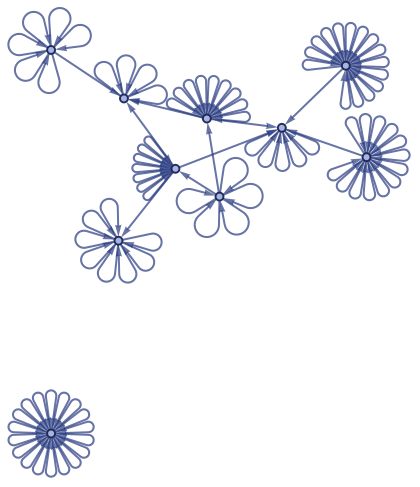
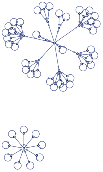
We have implemented a function which evolves the hypergraph until it becomes disconnected/a state is isomorphic to the next one/rule cannot be applied.
Dimension evolution
Dimension evolution
Mean Vertex Connectivity
Mean Vertex Connectivity
Some rules, like 245, 489, and 490 lead to long, seemingly fluctuating decay with a plateau at the end of the evolution. One could suspect that in the limit of large initial conditions such rules would create a halting mechanism for the universe.
Rule 234 leads to oscillations between the initial and the next step.
Rule 234 leads to oscillations between the initial and the next step.
The eight rules that behave like the rule 26, with a short and smooth evolution, fit a quasi-hyperbolic decay.
The states plots list helps us understand the decay better. For clarity, the initial condition has 3 vertices only.
The rule 245 evolution does not obey a simple smooth fit. During its evolution new vertices are not added and we are left with the final state.
Rule 245 halts shortly above 100 steps. For larger initial condition this takes place much further into the evolution. It is a busy beaver-type rule, leading to dimensional decay with fixed asymptotic dimension! This behaviour is in qualitative agreement with observed universe. High connectivity of the early universe explains the thermal equilibrium seen in the CMB. Currently, however, the number of spatial dimensions is fixed to 3.
We may wonder how robust these findings are. Starting with larger initial conditions (fully connected 20 vertices), we find similar decay shape for the rules 245, 489, and 26. Going to even larger initial conditions becomes computationally demanding.
One may, however, consider larger initial conditions which are not fully connected. This way we will see whether the connectivity decay depends on internal structure of the initial condition.
Random Initial Condition
Random Initial Condition
We consider a random sample of edges in a fully connected hypergraph e.g. choosing 300 edges from fully connected graph with 50 vertices
Sampling of low number of the edges will result in a lower number of vertices. This way we are not limited to a fixed number of vertices. We take such randomly generated initial condition and investigate its mean vertex connectivity for a set of rules.
There are now additional hypergraphs with periodic behaviour of period 3, seemingly random distributions around fixed dimension (seemingly, as there is a possibility of decay in much larger time scales. Rule 488 jumped form mean connectivity 11 to mean connectivity 6 in just one step!). There are still rules which result in connectivity decay (e.g. 245, 490).
Hausdorff dimension decay
Hausdorff dimension decay
We finally proceed to the discussion of Hausdorff dimension decay. As we will show, our results from the mean vertex connectivity section qualitatively hold.
Fully connected initial condition
Fully connected initial condition
We start with fully connected initial condition of 10 vertices. Hausdorff dimension evolution of the interesting rules is very similar to the mean vertex connection investigations. The differences are mostly in scaling of the Y-axis.
Randomly connected initial condition
Randomly connected initial condition
Let us show how does the dimensional decay changes with random initial conditions of the same mean connectivity. We plot mean Hausdorff dimension decay of rule 489 for 10 random initial conditions with 500 edges.
Dimensional decay is not sensitive to the change of the internal structure of initial condition, if all samples have the same mean connectivity. Moreover, even a drastic change (checked for rule 245 and initial hypergraph with 50 vertices and {1000, 2000, 2500} edges out of 2500 possible) in the connectivity of the initial condition does not change the fact that there is dimensional decay. Changes in mean connectivity impact initial and final dimension of the hypergraph.
We check numerically that Hausdorff dimension is a monotonically growing function of mean vertex connectivity. For rule 490 and the same random initial condition we have:
Outlook
Outlook
There is still a lot to figure out with dimensional decay in the Wolfram Model. Here are my suggestions:
◼
Are there limit manifolds? We’ve seen that asymptotically constant dimension is a general feature of certain rules, however, they do not produce manifold-like hypergraphs.
◼
How does the dimension decay connects to the shrinking speed of light idea? Variable speed of light is an alternative to cosmological inflation. In the context of Wolfram Model it seem to appear naturally in the causal graphs.
◼
Scalar field evolution on dimensionally decaying hypergraphs.
Keywords
Keywords
◼
Inflationary cosmology
◼
Quantum gravity
◼
Dimensional decay
◼
Hausdorff dimension
Acknowledgements
Acknowledgements
This project wouldn’t be possible without the invaluable help of my mentors- Jonathan Gorard and Cameron Beetar, who spent countless hours patiently explaining every detail in Wolfram Model and Wolfram Language. They are extremely competent and hard working. They have wonderful sense of humor and it was always fun to be around them.
I’d like to mention that it was a pleasure to be part of the student group mentored by Jonathan and that I will deeply miss them once the WSS2021 ends.
I’d like to mention that it was a pleasure to be part of the student group mentored by Jonathan and that I will deeply miss them once the WSS2021 ends.
References
References
◼
PLANCK Collaboration https://www.aanda.org/articles/aa/full_html/2020/09/aa33880-18/aa33880-18.html
◼
Stephen Wolfram, Wolfram Physics Project https://writings.stephenwolfram.com/2020/04/finally-we-may-have-a-path-to-the-fundamental-theory-of-physics-and-its-beautiful/