This problem was first given in Ref. 1 and solved with Excel. Here, we present the same problem but solved using FindRoot. We consider a steady-state pumping system with a branched pipe network (as shown below), where a centrifugal pump delivers water from a supply tank to two discharge tanks through three pipes. We propose to determine the unknown pressures at intermediate nodes, p2 and p3, as well as the flow rates in each pipe, QA, QB and QC.The elevations of all nodes (z1, z2, z3, z4 and z5) and the geometric characteristics of each pipe (length, diameter, friction factor) are known. The pressures at nodes 1, 4, and 5 are specified (atmospheric).
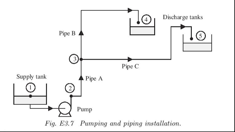
The problem is solved using three key principles: mechanical energy balances, continuity equation and pump empirical characteristic.
● For each pipe, the mechanical energy balance (including friction losses) is written as:with f the friction factor, C1=4636 and C2=4.01 when z (ft), p (psi), Q (gpm), L (ft), D (in), g (ft/s2) and ρ (lbm/ft3)
Δz+C1+g=0
Δp
ρg
C2fL
2
Q
5
D
● At node 3, conservation of mass requires: QA = QB + QC. This ensures that total inflow equals total outflow at the branching point.
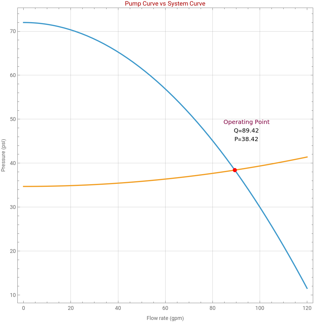
● The pump adds energy to the system according to an empirical characteristic: . In fact, pressure rise provided by the pump decreases with increasing flow rate due to internal hydraulic losses.
p2-p1=a-b
2
Q
Finally, we get a system of five nonlinear equations withfive unknowns: p2, p3, QA, QB, QC. These equations are solved simultaneously using FindRoot in Mathematica.
This problem illustrates how flow distribution in a network is governed by hydraulic resistance. Although Pipes B and C have the same diameter (i.e., DB=DC=2.067), their different lengths result in unequal flow splitting. The pump determines the total flow rate, while the network dictates how that flow is divided.
This problem illustrates how flow distribution in a network is governed by hydraulic resistance. Although Pipes B and C have the same diameter (i.e., DB=DC=2.067), their different lengths result in unequal flow splitting. The pump determines the total flow rate, while the network dictates how that flow is divided.
The solution, given at the end of this notebook, represents the intersection between: the pump curve (energy supplied) and the system curve (energy required). It is indicated in red and called the operating point. For the system curve, a simplification (i.e., an approximate approach) is used: where + Pstatic=ρ g z4 and K is adjusted as needed so that the two curve intersect at the operating point.
The analysis uses simultaneous application of energy balances, continuity, and equipment performance equations (i.e., pipe performance). Because of the nonlinear dependence on flow rate, a numerical approach based on FindRoot becomes handy.
K+Pstatic
2
Q
The analysis uses simultaneous application of energy balances, continuity, and equipment performance equations (i.e., pipe performance). Because of the nonlinear dependence on flow rate, a numerical approach based on FindRoot becomes handy.
Elevation
z1=0;z2=0;z3=25;z4=80;z5=60;
Gauge pressure - fluid is at atmospheric pressure
p1=0;p4=0;p5=0;
Pump characteristics
a=72;b=0.0042;
Assume these friction factors
fA=0.00523;fB=0.00584;fC=0.00556;
Pipes’ diameters
DA=3.068;DB=2.067;DC=2.067;
Pipes’ lengths
LA=80;LB=300;LC=500;
Water density
rho=62.4;
In ft/s2
g=32.2;
Constants
C1=4.636*10^3;C2=4.01;
Governing equations
eq1=(z3-z2)+C1*(p3-p2)/(rho*g)+C2*(fA*QA^2*LA)/(g*DA^5)==0;eq2=(z4-z3)+C1*(p4-p3)/(rho*g)+C2*(fB*QB^2*LB)/(g*DB^5)==0;eq3=(z5-z3)+C1*(p5-p3)/(rho*g)+C2*(fC*QC^2*LC)/(g*DC^5)==0;eq4=QA-QB-QC==0;eq5=p2==p1+a-b*QA^2;
Solve using FindRoot
sol=FindRoot[{eq1,eq2,eq3,eq4,eq5},{{p2,30},{p3,20},{QA,80},{QB,30},{QC,50}}];p2sol=p2/.sol;p3sol=p3/.sol;QAsol=QA/.sol;QBsol=QB/.sol;QCsol=QC/.sol;
Print["pressures:"];Print["p2 = ",NumberForm[p2sol,{6,2}]," psi"];Print["p3 = ",NumberForm[p3sol,{6,2}]," psi"];
Print["\nFlow rates:"];
Print["QA = ",NumberForm[QAsol,{6,2}]," gpm"];Print["QB = ",NumberForm[QBsol,{6,2}]," gpm"];Print["QC = ",NumberForm[QCsol,{6,2}]," gpm"];
Print["\nCheck continuity:"];
Print["QA ≈ QB + QC → ",NumberForm[QAsol,{6,2}]," ≈ ",NumberForm[QBsol+QCsol,{6,2}]];
pressures:
p2 = 38.42 psi
p3 = 26.92 psi
\nFlow rates:
QA = 89.42 gpm
QB = 35.06 gpm
QC = 54.36 gpm
Checkcontinuity:
QA ≈ QB + QC → 89.42 ≈ 89.42
To be adjusted as needed
K=0.0004649;
Approximately equal to rho*g*z4
Pstatic=34.7;
In[]:=
pump[Q_]:=a-bQ^2;
In[]:=
system[Q_]:=KQ^2+Pstatic;
Operating point
sol=FindRoot[pump[Q]-system[Q]==0,{Q,80}];
Qop=Q/.sol;Pop=pump[Qop];
Plot{pump[Q],system[Q]},{Q,0,120},
Out[]=


References
References
[1] J. O. Wilkes, Fluid Mechanics for Chemical Engineers, 2nd edition, NJ: Prentice Hall, 2006
CITE THIS NOTEBOOK
CITE THIS NOTEBOOK
Numerical solution of a complex piping system
by Housam Binous and Ahmed Bellagi
Wolfram Community, STAFF PICKS, April 23, 2026
https://community.wolfram.com/groups/-/m/t/3701079
by Housam Binous and Ahmed Bellagi
Wolfram Community, STAFF PICKS, April 23, 2026
https://community.wolfram.com/groups/-/m/t/3701079