Wolfram Cloud Document

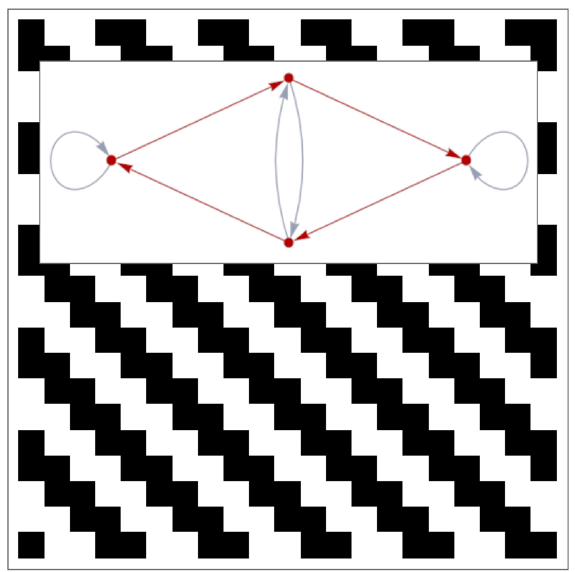
Generalized Ising models form a rich area in which one can explore questions of computability and of phase transitions [1]. While numerical methods to approximate ground states are readily available, few sources enumerated and prove the existence of periodic ground states in the thermodynamic limit. In this project, we follow the branch and bound paradigm for bounding the ground state from above [4], and we employ linear optimization with appropriate constraints for bounding the ground state from below [2]. When these bounds are equal, we have provably found a ground state in the thermodynamic limit. By employing general methods especially those described in Huang et al. 2016, this can be done for a surprisingly general class of generalized Ising models.

1. Introduction

The Ising model can be studied under many different contexts. In this article, we concern ourselves with the ground states of generalized Ising models on the square lattice.

The standard Ising model is described by the following energy function:

H[s]-J

∑

〈ij〉

where the variables

are called spins and take values from the set

{-1,1}

and the notation

〈i j〉

means that the sum is taken over all edges.

is often referred to as the Hamiltonian, but we should note that it doesn’t share any of the analytic or symplectic structure from classical mechanics.

For an

grid, we can define the ground state energy per site:



min

{s}

H[s]

We’re interested in the thermodynamic limit

N→∞

and

M→∞

. For the standard Ising model in two dimensions the ground state is simple: if

J>0

this is referred to as the ferromagnetic Ising model, and the two ground states are

for all

=-1

for all

. If

J<0

, then this is the antiferromagnetic Ising model and the ground states take on a checkerboard pattern. The ground state energy per site is

-2J

in both cases.

In a generalized Ising model, finding the ground state isn’t so easy! For example, what is the ground state of the following one-dimensional Ising model in the thermodynamic limit?

H[s]-

∑

(-2

i+1

i+2

i+1

i+2

i+1

i+3

i+4

i+5

)

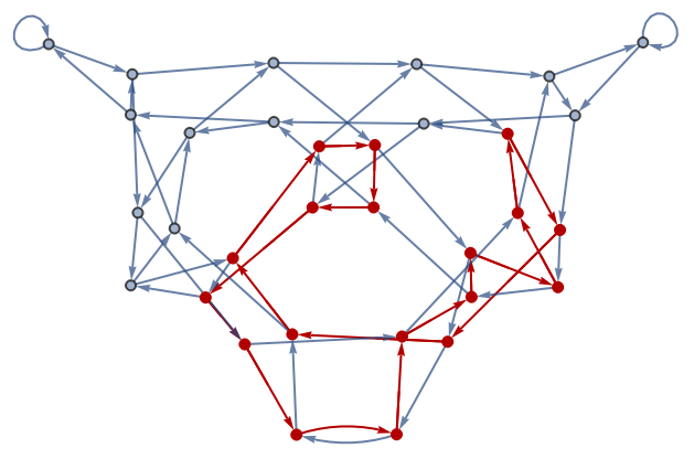
This seems like a difficult problem, but the literature is full of algorithms to solve for these ground states. Section 2 of this post covers the implementation of the function findIsingGS1D. In this particular case the ground states happen to have period 18 and energy per site -19/12.

In[]:=

example1=findIsingGS1D[{jCoef[1]-2,jCoef[2]-1,jCoef[1,1]-1/4,jCoef[1,2,1,1]1}];example1["energy"]{example1["GS"]//Length,example1["GS"]}

Out[]=

{18,{1,1,1,-1,1,-1,-1,1,1,-1,-1,1,-1,1,-1,1,1,-1}}

and the ground state corresponds to an 18-cycle through a particular graph:

In[]:=

example1["graph"]

Out[]=

It’s worth noting that the function findIsingGS1D doesn’t take care to include all possible ground states. findIsingGS1D finds a lowest energy state, but the following example only finds the ground state corresponding to

even though

=-1

is also a ground state.

In[]:=

example2=findIsingGS1D[{jCoef[1]1}];example2["energy"]{example2["GS"]//Length,example2["GS"]}

Out[]=

-1

Out[]=

{1,{1}}

1.2. Specifying the Generalized Model Programmatically

We consider Hamiltonians with n-spin interactions and translation invariance. A convenient way of specifying the Hamiltonians of this form is through a list of rules. By default the rules should all have head jCoef, and we can then pass these rules into our functions for finding ground states and energies.

In one dimension, if we want a nearest-neighbor spin-spin interaction to have a magnitude of j1, we specify the rule jCoef[1]->J1, corresponding to a term in the Hamiltonian

i+1

. Similarly, a rule jCoef[2]->J2 corresponds to terms like

i+2

. For three- and four-spin interactions, we keep adding arguments to jCoef. For example, the rule jCoef[1,1]->J11 corresponds to a term

1,1

i+1

i+2

, and in general a rule jCoef[a,b] corresponds to a term proportional to

i+a

i+a+b

In two dimensions, we could specify the two dimensional ferromagnetic Ising model with the rule list {jCoef[{0,1}]->J,jCoef[{1,0}]->J}. Each direction has to be specified separately, and this notation makes it very convenient to specify Hamiltonians such as the one studied in a previous summer school project [5]:

In[]:=

jRulesExample1={jCoef[{1,0}]->w1,jCoef[{0,1}]->w2,jCoef[{1,1}]->w4,jCoef[{1,-1}]->w3};With[{sizeN=2,sizeM=2},isingHamiltonian2D[sizeN,sizeM,Array[spin,{sizeN,sizeM}],jRulesExample1]]

Out[]=

-2w2spin[1,1]spin[1,2]-2w1spin[1,1]spin[2,1]-2w3spin[1,2]spin[2,1]-2w4spin[1,2]spin[2,1]-2w3spin[1,1]spin[2,2]-2w4spin[1,1]spin[2,2]-2w1spin[1,2]spin[2,2]-2w2spin[2,1]spin[2,2]

One slight difference in the 2D notation is that the difference vectors are not additive. For example, if a and b are 2D vectors, then the rule jCoef[a,b]->Jab corresponds to a term in the Hamiltonian that looks like

a,b

i+a

i+b

. jCoef[b,a]->Jab will correspond to the same term; the order of the arguments doesn’t matter. For example, here we define a four-spin interaction on a 2 by 2 lattice with periodic boundary conditions:

In[]:=

jRulesExample1={jCoef[{0,1},{1,0},{1,1}]1};With[{sizeN=2,sizeM=2},isingHamiltonian2D[sizeN,sizeM,Array[spin,{sizeN,sizeM}],jRulesExample1]]

Out[]=

-4spin[1,1]spin[1,2]spin[2,1]spin[2,2]

1.3. An Aside on the Presence of Higher Order Couplings

One question commonly crops up when studying such models: why do we care about three-spin interactions like

i+1

i+2

when the Ising model with its two-spin interactions got us so far? There are two ways that higher order interactions naturally arise:

When modeling a complex system, the true system involves many degrees of freedom while our effective Hamiltonian (aka our toy model) has just a few. When we average over the microscopic degrees of freedom so that one configuration of the effective Hamiltonian has to account for many configurations in the true system, we naturally find these higher order terms arising. (In statistical mechanics and field theory calculations this often arises through some calculation of the form

eff

T

∑

states

true

. If

true

only depends on pairwise interactions, solving the equation for

eff

can still give rise to much more exotic couplings).

It is a crucial aspect of the study of emergent properties of systems that we shouldn’t take the microscopic details of a toy model so seriously. Rather, we should analyze and classify universal behavior resulting from the toy model and extract real physical quantities from this universal behavior. If we throw out higher order terms, we might also throw out new emergent phenomena.

2. Finding Ground States in One Dimension

2.1. The Problem of Bounding Above and Below

How do we tackle the computational problem of finding the ground state of an infinite one-dimensional generalized Ising model? To make this concrete, let’s look at Hamiltonian

H-

∑

i+1

-2

i+2

. We could enforce periodic boundary conditions on a finite lattice with number of sites

sites

and find the ground state of this finite model. When we do this, we find that this particular model achieves a minimum energy whenever the number of sites is a multiple of 4:

Out[]=

	Upper Bound
	Lower Bound?

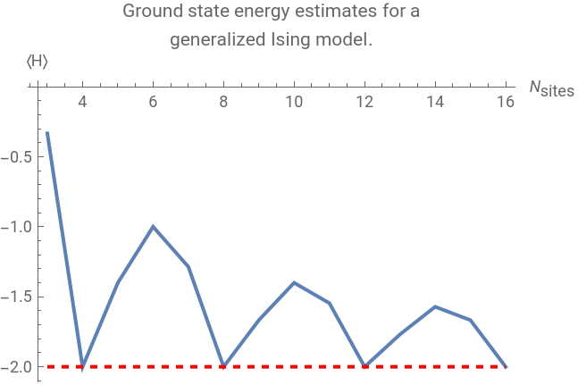
This strongly hints that the ground state energy equals

-2.0

with a period of 4, but all that we’ve proved is that the ground state energy is equal to or less than this energy. Finding a ground state with periodic boundary conditions gives us an upper bound for the ground state energy, and in two dimensions one must spend a large amount of computational effort on this step. Still, it’s only half of the battle! The other half is finding a lower bound for the ground state energy.

For this project, we implemented some of the algorithms from Huang et al. 2016 in Mathematica. Here we see that the ground state has periodicity 4, energy-per-site -2, and cycles like {1,1,-1,-1,...} forever. The energy of “-2” is exact, not just a lower or upper bound.

In[]:=

findIsingGS1D[{jCoef[1]->1,jCoef[2]->-2}]

Out[]=

energy-2,GS{1,1,-1,-1},graph

,rhoProbabilities



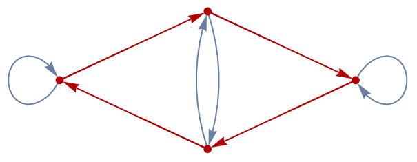
The method is lightning fast and it works for much more complicated Hamiltonians as well! In the example given previously with the 18-cycle, each vertex of the directed graph represents a possible five-state window (like {1,1,1,1,1}), and connections between vertices are only possible if you can get from one to the other by sliding your window to the right by one (so {1,1,1,1,1} has edges to {1,1,1,1,1} and {1,1,1,1,-1}.

We reserve a more full explanation of the algorithm in Huang et al. for a later date or a separate post. Critically, I have not covered the “compatibility conditions” needed to fully specify the optimization problem.

3. Finding Ground States in Two Dimensions

3.1. Changes to the Algorithm

In two dimensions we take a similar approach, and our algorithm can now spit out probabilities that specific N by M configurations occur. The pair (N,M) is called the block size, and we are met with three difficulties:

There might be no state that satisfies the appearance probabilities given from our algorithm. This means that unlike in one dimension, we might find a lower bound on the ground state energy which is not tight.

Because we lose the ability to construct a state from the appearance probabilities, this means that we lose our upper bound as well!

Point 2 can be tackled by taking the block size to be larger.

Point 3 can be tackled by finding explicit examples of low energy states through the branch and bound method. I found a Wolfram Community post by Daniel Lichtblau to be extremely helpful on this point [4].

For the purposes of this article, I don’t overcome point 1 and stick to small block sizes. 4 by 5 is the largest that we use in this article, though slightly larger block sizes could be tackled by optimizing the code and symbolic algebra. Huang et al. were able to overcome these difficulties by employing an algorithm called cluster tree optimization, and we leave a Mathematica implementation of that to future work.

3.2. Application to Various Systems

The code implementation in this notebook is robust enough to form the core backbone of an automated search for classifying ground states of 2D generaliezd Ising systems, but unfortunately the deadline for posting this article has arrived!

These tools were meant so that we can start exploring large combinations of coupling constants in an automated fashion, and this article won’t be considered complete until we edit it later with the results of this search.

3.3. Further Work

There are several areas for improvement.

◼

We can improve the upper bound finding algorithm. While the branch and bound code adapted from Daniel Lichtblau’s post [4] was extremely helpful, our adaptation is not as robust as it could be.

◼

We can implement the tree algorithm from Huang et al. [2]. This will be especially useful once we find coupling constants whose upper and lower bounds truly don’t converge after an exhaustive search on small block sizes.

4. Concluding Remarks

This concludes an exploration into the ground states of generalized Ising systems. While the algorithms implemented in this paper are not novel, we hope to make the larger philosophy of this type of investigation clear. First, we visualize results and algorithms to ensure that we have an eye into what our algorithms are doing. Second, we develop powerful automated tools to solve large classes of problems. Third, we apply these automated tools and specifically search for cases where our tools fail to solve the problem. These failure cases are likely the most interesting cases! Studying these failure cases for the generalized Ising model will have to be left to a future post, or future edit to this post.

Source Code

Acknowledgments

The author would like to thank Stephen Wolfram for suggesting this project, Nikolay Murzin and Sotiris Michos for thoughtful discussions on the specific ideas to implement, and the Wolfram Summer School team for hosting another fantastic program.

References

S. Wolfram (1985), “Undecidability and intractability in theoretical physics,” Physical Review Letters. https://www.doi.org/10.1103/physrevlett.54.735

W. Huang et al. (2016), “Constructing and proving the ground state of a generalized Ising model by the cluster tree optimization algorithm,” arXiv [cond-mat.stat-mech]. arXiv:1606.07429

A. Grabovsky (2017), “Construction of the ground state in the generalized Ising model,” Wolfram Community. https://community.wolfram.com/groups/-/m/t/1137293

D. Lichtblau (2016), response to “Solve an integer programming problem with LinearProgramming?” Wolfram Community. https://community.wolfram.com/groups/-/m/t/967349

Cite This Notebook

“Finding and bounding generalized ising model ground state energies”
by David Moore
https://community.wolfram.com/groups/-/m/t/3211260