This project uses the Wolfram Language to simulate how a particle beam travels through a series of magnets. Moving up from a simpler 2 by 2 matrix that only tracks one plane, this simulation uses 4 by 4 matrices to calculate horizontal and vertical positions and angles at the same time. A beam of 9,000 particles was created using a Gaussian distribution. The particles were first sent through a 1-meter drift space to see how they spread out, which was plotted using hexagonal density bins. Next, the beam was tracked through a symmetric FODO focusing channel for 5 turns. By calculating the standard deviation of the tracking data, the horizontal and vertical beam sizes (, , , ) were plotted to show how the alternating magnets keep the beam focused. This simulation provides a working framework that can be expanded to test more advanced types of magnets in the future.
σ
x
σ
x'
σ
y
σ
y'
Introduction
Introduction
In modern high-energy physics, particle accelerators serve as vital instruments for investigating fundamental interactions by accelerating charged particles to near-light speeds and colliding them. Managing these high-energy beams requires extraordinary precision. Within an accelerator beamline, particles are guided, focused, and steered using specialized magnetic fields. Because full-scale particle simulations involving thousands of distinct magnetic components are computationally demanding, linear beam dynamics utilizes a modular matrix framework to track single particles and coordinate distributions across successive beamline components.
This project aims to develop a computational simulation framework in the Wolfram Language to model and track particle beam optics across modular accelerator components. By implementing 2×2 and 4×4 transfer matrices, the tools simulate transverse particle trajectories and phase space stability through multi-element periodic lattices. This framework replaces resource-intensive numerical integration with discrete matrix transformations to evaluate beamline focusing configurations.
The computational essay is organized as follows: Section 2 covers the mathematical theory of transfer matrices, demonstrates matrix multiplication closure for drift spaces, and explains focal sign behaviors in quadrupole lenses. Section 3 details the Wolfram Language implementation for both the 2×2 dipole-drift models and 4×4 quadrupole lines, explicitly stepping through code blocks and tracking outputs. Section 4 summarizes our findings, followed by potential future research directions.
Theory
Theory
Ray Tracing and Transfer Matrices
Ray Tracing and Transfer Matrices
The motion of charged particles with respect to the center of the beam pipe in an accelerator conceptually resembles the motion of optical rays with respect to the optical axis. In a single transverse plane (such as the horizontal plane ), a particle's spatial configuration at any point along the longitudinal track coordinate is fully defined by its lateral displacement x and its divergence angle .Assuming linear forces, the transformation of this coordinate vector from an initial position to a subsequent position can be described by a linear operation—a matrix multiplication. The final coordinates, denoted with a hat symbol , ), are computed from the initial coordinates across a beam element via a 2×2 linear transformation matrix, known as the transfer matrix:
R·
x
s
′
x
dx
ds
(
x
′
x
(x,)
′
x
x |
′ x |
x |
′ x |
R 11 | R 12 |
R 21 | R 22 |
x |
′ x |
This matrix equation handles single-particle tracking elegantly: the elements and determine the downstream position = + , while and determine the downstream divergence angle = x + .
R
11
R
12
x
R
11
R
12
′
x
R
21
R
22
′
x
R
21
R
22
′
x
Closure of Matrix Multiplication (Drift Space Example)
Closure of Matrix Multiplication (Drift Space Example)
An essential requirement of linear beam optics is that successive applications of transfer matrices within the same physical category must preserve their algebraic form. To demonstrate this closure property, consider a drift space of length , which contains no magnetic fields. A particle traveling through this space preserves its angle ( = ), while its position changes linearly according to = + . The transfer matrix for a drift length is written as:(L)
L
′
x
′
x
x
x
L
′
x
L
M
drift
1 | L |
0 | 1 |
If a particle passes through two consecutive drift sections of lengths and , the net effect is found by multiplying their corresponding matrices:()·()
Because = (+), the matrix multiplication is closed under this operation. The algebraic shape of the equation remains unchanged, confirming that splitting a drift space into arbitrary subdivisions does not alter the underlying transport physics.
d
1
d
2
M
total
M
drift
d
2
M
drift
d
1
1 | d 2 |
0 | 1 |
1 | d 1 |
0 | 1 |
M
total
(1·1+ d 2 | (1· d 1 d 2 |
(0·1+1·0) | (0· d 1 |
1 | d 1 d 2 |
0 | 1 |
M
total
M
drift
d
1
d
2
The Transition from 2×2 to 4×4 Matrix Mechanics
The Transition from 2×2 to 4×4 Matrix Mechanics
While a 2×2 matrix effectively models movement within a single isolated dimension, real accelerators require simultaneous tracking of both horizontal (, ) and vertical ( , ) coordinates. When the horizontal and vertical motions are uncoupled—meaning fields in the direction do not depend on or alter motion in —the system can be represented by a 4×4 block-diagonal matrix that relates the initial state to the final state (,, , ):
·
For an uncoupled 4×4 drift space, the matrix expands to combine the independent horizontal and vertical sub-drift matrices:(L)
x
′
x
y
′
y
x
y
x
′
x
y
′
y
x |
′ x |
y |
′ y |
R
4×4
x |
′ x |
y |
′ y |
R 11 | R 12 | 0 | 0 |
R 21 | R 22 | 0 | 0 |
0 | 0 | R 33 | R 34 |
0 | 0 | R 43 | R 44 |
x |
′ x |
y |
′ y |
M
drift4
1 | L | 0 | 0 |
0 | 1 | 0 | 0 |
0 | 0 | 1 | L |
0 | 0 | 0 | 1 |
Quadrupole Lenses and Sign Asymmetry
Quadrupole Lenses and Sign Asymmetry
A quadrupole magnet produces a magnetic field that increases linearly with distance from the central axis . This field profile exerts a focusing force in one transverse plane while simultaneously acting as a de-focusing force in the orthogonal plane . Under the thin - lens approximation, where the magnet length approaches zero while maintaining a constant integrated field strength, a quadrupole lens alters only the divergence angle of the incoming particles, leaving their transverse positions unchanged ( = and = ) . In a 4 by 4 thin - lens matrix formulation, the lens transformation is defined by :
(f)·
This matrix highlights an essential characteristic of quadrupole lenses: the opposite sign convention between the horizontal and vertical focusing elements. If the lens is configured to focus the beam horizontally (=-1/f forces divergent rays back toward the center axis so that =-x/f+x' ), Maxwell’s equations dictate that it must defocus the beam vertically (=1/f drives particles away from the axis so that =-y/f+y'). Consequently, a single quadrupole cannot focus a beam in both planes simultaneously.
x
x
y
y
x |
′ x |
y |
′ y |
M
quad4
x |
′ x |
y |
′ y |
1 | 0 | 0 | 0 |
- 1 f | 1 | 0 | 0 |
0 | 0 | 1 | 0 |
0 | 0 | 1 f | 1 |
x |
′ x |
y |
′ y |
R
21
x'
R
43
y'
Periodic Focusing and the FODO Cell Lattices
Periodic Focusing and the FODO Cell Lattices
To achieve net focusing and stable containment in both dimensions over long distances, accelerators utilize a periodic arrangement of alternating lenses known as a FODO lattice. A single FODO cell forms the fundamental building block of an accelerator line. The name represents the physical sequence of its components:
◼
F: A focusing quadrupole lens (which focuses the beam in the horizontal plane, while de-focusing in the vertical plane).
◼
O: A drift space (free space allowing the beam to coast).
◼
D: A de-focusing quadrupole lens (which de-focuses the beam in the horizontal plane, while focusing in the vertical plane).
◼
O: A second drift space.
By alternating these elements, a particle that receives a de-focusing kick from one lens arrives at the next lens with a larger displacement from the axis, where it experiences a proportionally stronger focusing kick. This alternating gradient structure creates a net restoring force in both planes simultaneously, keeping the particle beam confined inside the vacuum chamber over indefinitely long propagation distances.
Simulation
Simulation
To systematically evaluate the tracking layout, the computational simulation framework is split into two development stages. The first stage establishes a single-plane 2 by 2 matrix transfer model to isolate and verify horizontal transverse dynamics. Once this tracking logic is validated against known single-plane benchmarks, the framework expands into a unified 4 by 4 multi-plane architecture to handle simultaneous horizontal and vertical beam focusing.
2×2 Single-Plane Transport Code
2×2 Single-Plane Transport Code
To build the simulation framework, I first need to define the fundamental building blocks of an accelerator lattice as reusable matrix functions in the Wolfram Language. I set up the standard 2×2 transfer matrix for a drift space of length l to model free drift, alongside a thin-lens quadrupole matrix that applies an angular kick proportional to the particle’s displacement and the lens’s focal length f.
drift[l] constructs the 2 by 2 matrix for a field-free space of length l, while q[f] defines a thin-lens quadrupole matrix that modifies the particle’s divergence angle based on the focal parameter f:
In[]:=
drift[l_]:={{1,l},{0,1}};
In[]:=
q[f_]:={{1,0},{-1/f,1}};
To build a realistic simulation setup, the physical dimensions and focal parameters are configured to match standard baseline lattices from the CERN Accelerator School (CAS) Primer.
In[]:=
f=1;l=1/10.;beamLine=ConstantArray[drift[l],5]~Join~{q[-f]}~Join~ConstantArray[drift[l],10]~Join~{q[.84*f]}~Join~ConstantArray[drift[l],5];
I set the starting position (xInit) to simulate a particle that starts 2mm away from the center line (x) but is traveling completely straight with zero initial angle (x’).
In[]:=
xInit={0.002,0};
Because matrix multiplication is closed under linear coordinate transformations, any arbitrary arrangement or sequence of components can be mathematically compressed down into a single cumulative 2 by 2 transfer matrix.
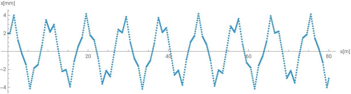
Using FoldList to repeat the cell 40 times:
In[]:=
output=FoldList[#2.#1&,xInit,Join@@ConstantArray[beamLine,40]];
To generate an accurate physical trajectory plot, the cumulative longitudinal coordinate () must be resolved by accumulating the physical thicknesses of each individual matrix element across the simulation path.
s
This block computes the precise longitudinal axis coordinate:
In[]:=
displacement=ConstantArray[l,5]~Join~{0}~Join~ConstantArray[l,10]~Join~{0}~Join~ConstantArray[l,5];displacement=Prepend[Accumulate[Flatten[ConstantArray[displacement,40]]],0];
Plots the transverse particle displacement as a function of the longitudinal position s:
In[]:=
ListPlot[{displacement,1000*output[[All,1]]}//Transpose,PlotRange->All,PlotStyle->PointSize[0.005],AspectRatio->1/4,AxesLabel->{"s[m]","x[mm]"}]
Out[]=
To analyze lattice stability boundaries and beam containment limits, an alternative configuration featuring longer drift lengths and altered focal strengths is evaluated.
In[]:=
f2=2.5;l2=0.2;
In[]:=
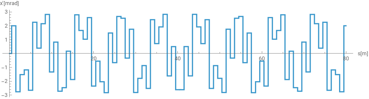
ListPlot[{displacement,1000*output[[All,2]]}//Transpose,PlotRange->All,PlotStyle->PointSize[0.08],AspectRatio->1/4,Joined->True,AxesLabel->{"s[m]","x'[mrad]"}]
Out[]=
Gaussian beam. Both position offset and incidence angle follows normal distribution:
To scale the project from single-particle tracking to collective beam dynamics, a statistical ensemble modeling a multi-particle Gaussian beam is generated. The initial coordinates are sampled using a bivariate normal distribution.
This code initializes a distribution of 9,000 discrete particles in phase space (x vs x’). It applies a customized binning function to visualize the particle density distribution as a localized phase-space ellipse:
Gaussian beam after one drift:
To study beam containment over long-term operations, a multi-particle tracking loop is implemented to evaluate the evolution of the coordinate distribution across repeated periodic structures.
This code block handles the multi-particle simulation across a secondary lattice structure. It initializes a 5-cell repetition sequence and implements a Table loop that maps the recursive tracking logic across every individual coordinate pair in the 9,000-particle ensemble:
9,000 copies of a list with 111 items, each item has 2 elements (x,x’):
Standard deviation of x and x prime of Gaussian Beams
Standard deviation of x and x prime of Gaussian Beams
Once the multi-particle tracking data array is populated, macro-level statistical properties of the beam can be extracted at each longitudinal position step along the accelerator axis.
4×4 Dual-Plane Quadrupole Tracking Framework
4×4 Dual-Plane Quadrupole Tracking Framework
To accurately capture coupling-free multi-plane particle tracking, the verified tracking logic from the single-plane 2 by 2 benchmark is expanded into a 4-dimensional state-space model. While the core algorithmic structure remains exactly the same as the 2 by 2 case, the model is scaled up to handle four independent variables simultaneously—tracking both horizontal (x, x’) and vertical (y, y’) spatial positions and divergence angles within a unified matrix system.
This cell expands the fundamental lattice data structures into 4 by 4 block-diagonal matrix functions:
To maintain structural consistency with the baseline single-plane validation tests, the FODO cell arrangement is constructed using matching element intervals and focal parameters.
Because tracking multi-plane motion requires a complete coordinate profile, the initial particle state must be updated to a 4-element vector containing independent horizontal and vertical parameters.
To maintain structural consistency with the baseline single-plane validation tests, the FODO cell arrangement is constructed using matching element intervals and focal parameters.
This cell initializes the 4-dimensional particle state vector xInit4D. It simulates an initial horizontal offset of 2mm with zero divergence, paired with an initial vertical offset of 5mm and an off-axis vertical divergence angle of 3mrad:
This cell executes the multi-plane iterative tracking routine over 40 lattice cells. Using FoldList, the code evaluates the 4-dimensional matrix-vector product recursively:
To plot the resulting trajectories alongside each other, the spatial coordinates are isolated from the multi-dimensional output array and mapped against the cumulative longitudinal path distance (s).
Pairs the calculated independent longitudinal position data vector (displacement) with the horizontal tracking spatial coordinate array (output[[All, 1]]), scaled by a factor of 1000 to convert the output axis into millimeters. The resulting plot displays the stable, alternating transverse betatron oscillations of the particle’s horizontal coordinate over the full length of the 40-cell magnetic transport channel:
To expand the multi-particle simulation into two dimensions simultaneously, a multi-dimensional coordinate distribution is generated. The initial state of the beam ensemble is modeled as a 4D Gaussian distribution in phase space.
This cell initializes a distribution of 9,000 discrete particles across four dimensions (x, x’, y, y’). The initial coordinates are randomly sampled from a multi-bivariate normal distribution, setting up independent, uncoupled horizontal and vertical phase-space ellipses:
This code generates a collective beam distribution vector containing 9,000 macroparticles using RandomVariate and MultinormalDistribution. The first argument defines the centroid offsets for each phase parameter (x, x’ , y, y’), while the second represents the diagonal covariance matrix defining the coordinate variances (beam size and divergence bounds):
To evaluate the transverse spatial density distribution prior to lattice injection, the tracking components are grouped and binned into hexagonal spatial arrays .
This code extracts the initial horizontal phase space components (x and x’ via [[All, ;; 2]]), partitioning the coordinate pairs into hexagonal density bins with a radius specification of 0.1. The distribution density is rendered visually by mapping cell population counts (Values[tiles]) to a scaled opacity range between 0 and 1 using a deep blue color filter:
This code isolates the corresponding vertical tracking components (y and y’ via [[All, 3 ;;]]) from the base macroparticle matrix. It computes their local phase space densities and displays them inside an independent two-dimensional grid array layout to establish the structural state of the incoming beam:
This code generates the 9,000-particle array across a 1-meter free drift section by evaluating the right-side matrix transformation product against Transpose[drift4[1]]. The subsequent horizontal density plot tracks the characteristic coordinate shearing effect, where forward longitudinal drift momentum translates position coordinates into an angled distribution profile:
This block of code computes and graphs the corresponding vertical plane density grid (tiles4) after the initial 1-meter drift transformation, confirming identical uncoupled linear drift expansion behaviors across both transverse axes:
A primary symmetric FODO channel configuration is declared using an altered lattice element scaling routine and tracking framework.
This sets up a master position timeline map array vector to trace progress along the total longitudinal transport span:
Runs a multi-particle structural loop via Table, passing every single drifted macro-particle vector b through 5 consecutive replications of our active beamLine2 element array sequence, yielding a comprehensive track file array recording history:
{1,0,0,0} represents that only the x value is needed.
This code extracts the companion statistical root-mean-square horizontal divergence distribution trajectory history (σ_x’(s)) by pulling out index parameter 2, mapping the geometric beam focus transformations taking place over the element transitions:
{0,1,0,0} represents the x’ value.
Conclusion
Conclusion
Future Directions
Future Directions
While the current linear, thin-lens framework provides an excellent benchmark for core accelerator physics behaviors, realistic beam lines demand higher-fidelity magnetic field representations and geometric variations. Future extensions of this computational framework will focus on the following core developments:
◼
Transition to Thick-Lens Formulations: The current thin-lens quadrupole approximation (q4[f]) applies an instantaneous angular kick to the particle’s divergence. To capture the true spatial transformations within a physical magnetic element, future iterations will implement thick-lens matrix operators
◼
Integration of Dipole Bending Magnets: To simulate true sector storage rings or transfer lines rather than straight transport channels, a $4\times4$ block-diagonal matrix for sector dipoles and rectangular dipoles will be introduced. This will incorporate geometric path bending in the horizontal plane alongside weak focusing effects.
◼
Coupling Elements (Skew Quadrupole): To investigate realistic alignment errors and multi-plane coupling, skew quadrupole elements—which rotate the magnetic poles by 45 degrees—will be integrated. This will populate the off-diagonal blocks of our 4 by 4 transfer matrices, enabling the simulation of physical emittance transfer between the horizontal and vertical planes.
References
References
◼
H. Wiedemann, Particle Accelerator Physics (2 vol.), Springer Verlag, Heidelberg, 1998.
◼
A. Wolski, Beam dynamics in high-energy particle accelerators, Imperial College Press, London, 2014.
◼
G. Sterbini, A. Latina, V. Ziemann, Solutions of the Exercises of the Transverse Linear Beam Dynamics Primer using Python.
◼
A Wolski, CI-BEAM-223 Single-Particle Dynamics, https://indico.stfc.ac.uk/category/88/
Acknowledgements
Acknowledgements
I would like to thank my mentor Shenghui Yang for guiding this project throughout the summer and for pushing me to understand the sign structure of the quadrupole matrix rather than just use it. I would also like to thank the Program Directors, the TAs, and Stephen Wolfram for the opportunity to work on this project.
Additional thanks to Stephen Wolfram for suggesting this project.
CITE THIS NOTEBOOK
CITE THIS NOTEBOOK
Matrix-based modeling of particle beam transport
by Aikumis Olzhas
Wolfram Community, STAFF PICKS, July 9, 2026
https://community.wolfram.com/groups/-/m/t/3754335
by Aikumis Olzhas
Wolfram Community, STAFF PICKS, July 9, 2026
https://community.wolfram.com/groups/-/m/t/3754335