Breakthrough curves for adsorption with longitudinal diffusion
Authors: Housam Binous and Ahmed Bellagi
Breakthrough curves for adsorption with longitudinal diffusion
Authors: Housam Binous and Ahmed Bellagi
Authors: Housam Binous and Ahmed Bellagi
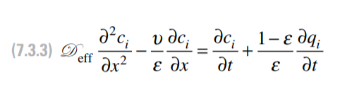
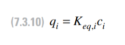
Acknowledgement: The expression for the analytical solution and the governing equations, for adsorption with longitudinal diffusion under equilibrium assumption, were obtained from Refs. 1 and 2.References:1- Harrison at al., Bioseparations Science and Engineering, Oxford University Press, 2003.2- Leon Lapidus and Neal R. Amundson, "Mathematics of Adsorption in Beds. VI. The Effect of Longitudinal Diffusion in Ion Exchange and Chromatographic Columns", J. Phys. Chem., vol. 56, p. 984, 1952.
In[]:=
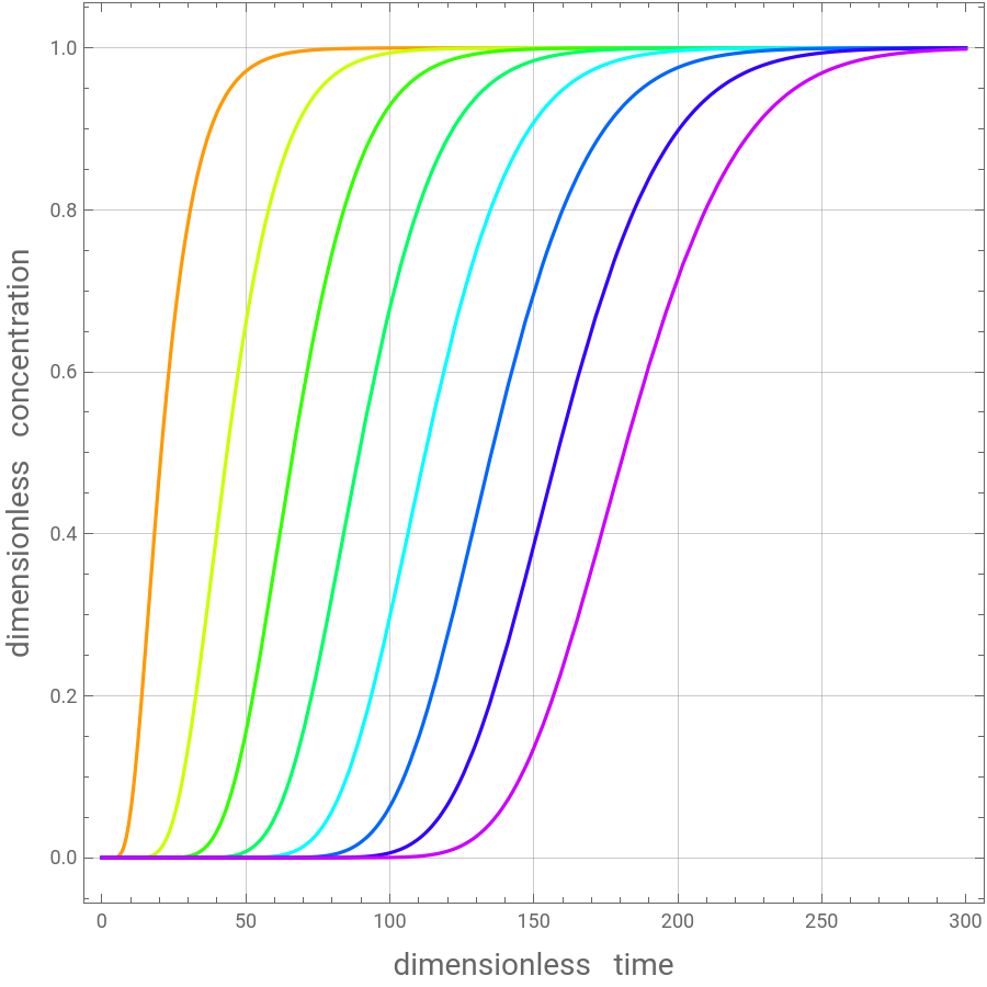
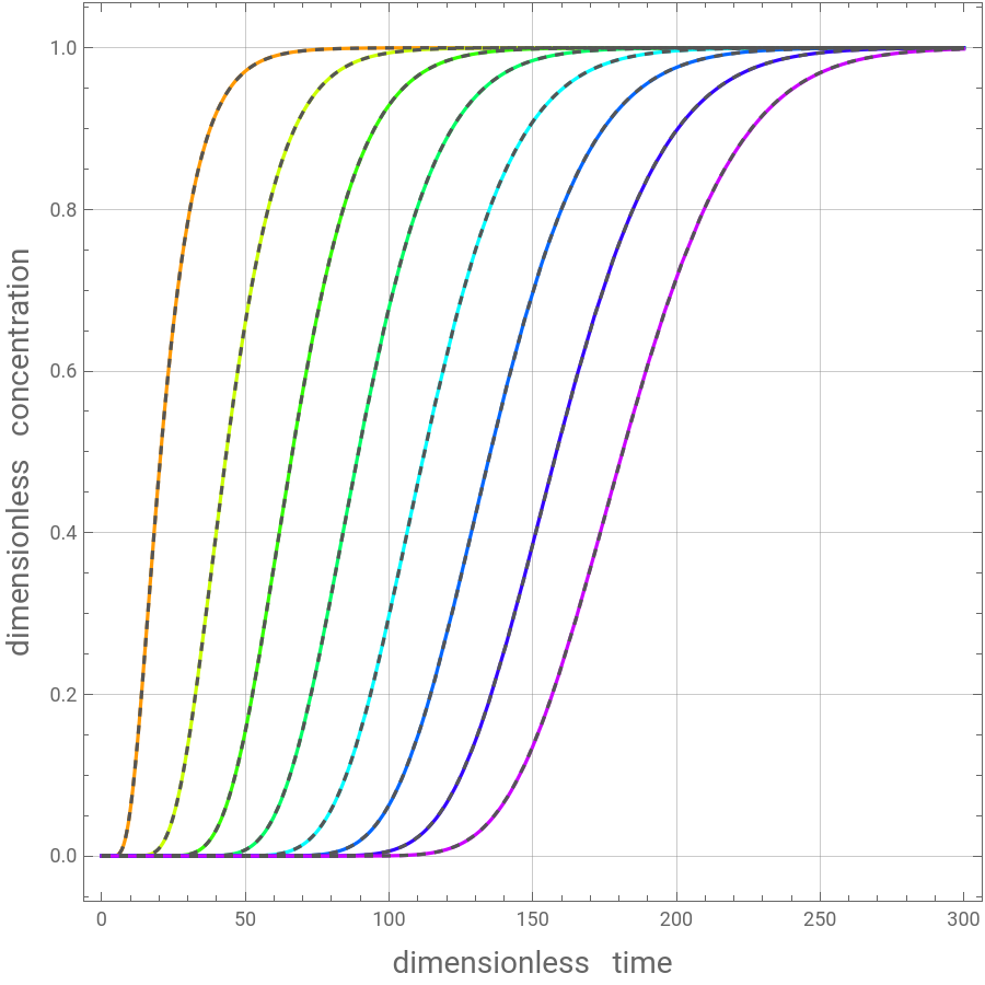
Numerical solution for the breakthrough curves for De=1.
Results obtained using NDSolve are identical to their counterparts using analytical derivation given in Harrison et. al. (2003) and Lapidus and Amundson (1952).
Results obtained using NDSolve are identical to their counterparts using analytical derivation given in Harrison et. al. (2003) and Lapidus and Amundson (1952).
In[]:=
Keq=10;Ka=1;V=1;De=1;α=0.6;
In[]:=
n[z_,t_]:=Keqc[z,t]
In[]:=
sol=NDSolve[{DeD[c[z,t],{z,2}]V/αD[c[z,t],{z,1}]+D[c[z,t],{t,1}]+(1-α)/αD[n[z,t],{t,1}],c[0,t]1,c[z,0]Exp[-1000z]},{c[z,t]},{z,0,50},{t,0,1000},Method{"MethodOfLines","SpatialDiscretization"{"TensorProductGrid"}},PrecisionGoal5]

Out[]=
c[z,t]InterpolatingFunction
[z,t]


In[]:=
p1=Show[Table[Plot[Evaluate[c[z,t]/.sol],{t,0,300},PlotRangeAll,PlotLegendsTable[Style[,Black],{i,3,20,2}],PlotStyleHue[z/50],AspectRatio1,ImageSize450{1,1},GridLinesAutomatic,FrameTrue,FrameLabel{Style["dimensionless time",14],Style["dimensionless concentration",14]}],{z,5,40,5}]]
c
z
Out[]=


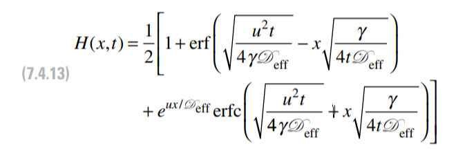
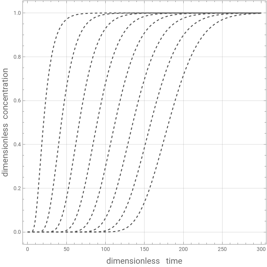
An analytical solution is available (see Ref. 1) :
In[]:=
γ=1+Keq(1-α)/α;Z=.;
In[]:=
u=V/α;
In[]:=
H1[t_]:=1/21+Erf
u^2t/(4γDe)
-Zγ/(4tDe)
+Exp[uZ/De]Erfcu^2t/(4γDe)
+Zγ/(4tDe)
In[]:=
p2=Show[Table[Plot[H1[t],{t,0,300},PlotRangeAll,PlotStyle{Darker@Gray,Dashed},AspectRatio1,ImageSize450{1,1},GridLinesAutomatic,FrameTrue,FrameLabel{Style["dimensionless time",14],Style["dimensionless concentration",14]}],{Z,5,40,5}]]
Out[]=
In[]:=
Show[p1,p2,PlotRange{{0,300},{0,1}},FrameTrue]
Out[]=
Numerical solution for the breakthrough curves for De=10.
Results obtained using NDSolve are identical to their counterparts using analytical derivation given in Harrison et. al. (2003) and Lapidus and Amundson (1952).
Results obtained using NDSolve are identical to their counterparts using analytical derivation given in Harrison et. al. (2003) and Lapidus and Amundson (1952).
In[]:=
De=10;
In[]:=
sol=NDSolve[{DeD[c[z,t],{z,2}]V/αD[c[z,t],{z,1}]+D[c[z,t],{t,1}]+(1-α)/αD[n[z,t],{t,1}],c[0,t]1,c[z,0]Exp[-10000z]},{c[z,t]},{z,0,100},{t,0,1000},Method{"MethodOfLines","SpatialDiscretization"{"TensorProductGrid","MinPoints"->10000}},PrecisionGoal5]
Out[]=
c[z,t]InterpolatingFunction
[z,t]
Effect of longitudinal diffusion on breakthrough curves.
Notice the curve shape change when ones goes from De=1 to De=10.
Notice the curve shape change when ones goes from De=1 to De=10.