The AdS/CFT correspondence defines an equivalence relation between d+2 dimensional anti-de Sitter (AdS) spaces and d+1 dimensional conformal field theories existing on the boundary of AdS space. AdS/CFT thus provides a framework for understanding the connection between general relativity and quantum field theory. In this project, we define the concept of a density matrix for string substitution systems to calculate the global entropy as well as the local entanglement entropy as a function of time and explore connections to the Bekenstein Bound. These tools provide a framework to help us in future investigations regarding the validity of the AdS/CFT duality within Wolfram models.
In future work we aim to define the density matrix of the vacuum state, thus allowing us to directly compute the Bekenstein Bound from the a measure relative entropy. We then hope to identify systems satisfying this bound and make conclusions based on our results. We seek to classify the nature of holographic surfaces within Wolfram models and calculate their areas to concretely relate the tools and findings developed in this work to the AdS/CFT correspondence. Moreover, we wish to investigate the origin of holographic gravity by relating it to causal invariance using the tools we have built.
In future work we aim to define the density matrix of the vacuum state, thus allowing us to directly compute the Bekenstein Bound from the a measure relative entropy. We then hope to identify systems satisfying this bound and make conclusions based on our results. We seek to classify the nature of holographic surfaces within Wolfram models and calculate their areas to concretely relate the tools and findings developed in this work to the AdS/CFT correspondence. Moreover, we wish to investigate the origin of holographic gravity by relating it to causal invariance using the tools we have built.
Introduction
Introduction
The AdS/CFT correspondence is possibly the most valuable clue that can guide us to a quantum theory of gravity. It predicts a unification of geometry (General Relativity) and quantum information (Quantum Theory). Remarkably, it predicts that the structure of space is defined by the information encoded on that space’s boundary surface.
Imagine space as an ocean with individual water molecules moving around in it. Collectively the water molecules give the sea it’s texture, waves, and all other properties. A single water molecule possesses none of these macroscopic properties. Look at the ocean waves for a brief moment in time. Now close your eyes and ask how many possible variations the ocean could exist while your eyes are closed. Without making any observation, the sea is in a superposition of all possible states. There is a geometrical structure that defines the correlations between all of these states. At any point in time, this is known as branchial space. By opening your eyes, you observe one of the many possible states and thus conclude the ocean is in a single state, ignoring all the complexity of quantum interference. As a macroscopic observer, we only follow one definite path through state space with time. The AdS/CFT correspondence states that our reality (in this case, the ocean behavior) can be described by a lot less information than one would classically expect. In the ocean analogy, it would suggest that the entire configuration of the ocean could, in a sense, be described by only observing its waves. In the same spirit, the description of the universe is entirely encoded on its boundary. And just like a hologram, the lower-dimensional description is projected onto a higher dimensional region.
This information is related to the existence of quantum states which describe all possible states of the universe. And crucially, the relationships between these states seem to define the force of gravity i.e., the structure of spacetime.
More precisely, AdS/CFT states that the physics of a negatively curved universe known as anti-de Sitter (AdS) space is encoded within a conformal field theory (CFT) existing on the area of its boundary. Inspired by the thermodynamic relationship between the area and the entropy (information) of a black hole first proposed by Bekenstein [1], Ryu and Takayanagi [2] (RT) generalized the correspondence to cosmological horizons essentially acting as a holographic screen [3]. In other words, the AdS/CFT correspondence relates the quantum states existing within state space (defined by the multiway causal graph) to the geometry of spacetime (represented by the causal graph) and in doing so postulates that the area of a geometric surface is defined by the entropy of quantum states describing it.
In this project, we try to build some of the necessary tools and intuitions required to investigate such correspondence within Wolfram models.
Bekenstein Bound
Bekenstein Bound
To understand the exact nature of AdS/CFT, we must first understand the microscopic details of the Bekenstein Bound, which defines a limit to the maximal amount of information (entropy) that can exist within a given region of space. It turns out that black holes exactly saturate this bound. One necessary component in understanding this bound is the density matrix describing the statistical ensemble of quantum states. We tried to develop a consistent way in which to define the density matrix. From the density matrix, one can compute a region’s entropy, which establishes the correlation between that region of space and the rest of space.
We will start by investigating the microscopic nature of the Bekenstein bound, which will act as a stepping stone towards AdS/CFT. Inspired by the generalized second law of thermodynamics, Bekenstein proposed the entropy bound:
Out[]=
S≤
2πER
ℏ
where S, E, and R are the entropy, energy, and radius of a system. Note that the bound is independent of the gravitational constant G.
A microscopic derivation of the Bekenstein Bound was first proposed by Casini [4] by considering the localized relative (vacuum subtracted) entropy of matter systems. Thus, we require a localized notion of energy, which in turn requires defining a local vacuum density matrix. The microscopic interpretation of the Bekenstein Bound is then the statement that the statistical distance between a localized state and its corresponding localized vacuum state must always be greater than zero. In more technical terms, the bound is enforced by requiring the positivity of the Kullback–Leibler divergence (relative entropy), which is directly related to the existence of a Fisher information metric describing quantum states.
Defining the Density Matrix in String Substitution Systems
Defining the Density Matrix in String Substitution Systems
To define the Bekenstein Bound in Wolfram models, we need to define several new concepts. First, we need a local entropy notion that measures the degree of entanglement (correlation) between local subsystems. Our initial attempt to calculate the entanglement entropy via the von Neumann entropy, considered decomposing the branchial graph, representing the relations between possible quantum states at any moment in time, into individual wavefunctions of all branch pairs (correlated states). From here, one can compute the global density matrix by summing over all wavefunctions of the system. Consider the following example of a complete branchial graph with five states (K_5) and ten branch pairs (edges) where vertex labels correspond to state path weights, which occurs after one time step. The rule for this system is “A”->”ABA”,”AA”->”B” and the initial condition is “AABAA”:
In[]:=
g=ResourceFunction["MultiwaySystem"][{"A""ABA","AA""B"},"AABAA",1,"BranchialGraph","IncludeStatePathWeights"True,VertexLabels"VertexWeight"]
Out[]=
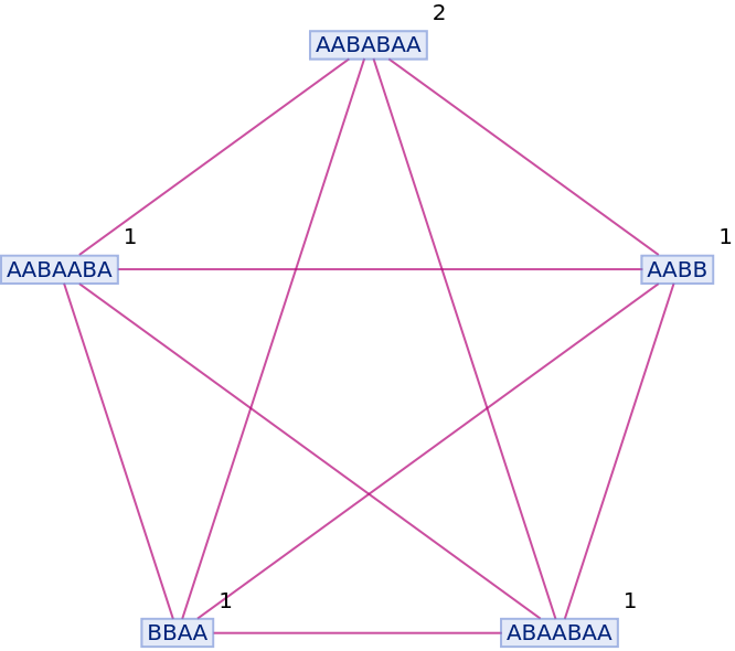
The corresponding list of branch pairs are given by:
Out[]=
{{AABAABA,AABABAA},{AABAABA,AABB},{AABAABA,ABAABAA},{AABAABA,BBAA},{AABABAA,AABB},{AABABAA,ABAABAA},{AABABAA,BBAA},{AABB,ABAABAA},{AABB,BBAA},{ABAABAA,BBAA}}
We propose that each branch pair be represented by a linear quantum superposition weighted by the corresponding probability amplitudes defined by the state path weights of each state. We can now compute the global density matrix by summing over all branch pair superpositions.
Notice, however, that some states are of varying length and thus have a different size Hilbert space associated with it. More specifically, the shorter states, “AABB” and “BBAA”, are defined by a Hilbert space which is a subspace of the Hilbert space of the remaining states. This may lead to issues in establishing a single global density matrix and requires further investigation.
Another approach to derive the global density matrix is to compute the branchial graph’s weighted adjacency matrix and include self connections. The magnitude of elements of this density matrix depends on the vertex weights. For the above branchial graph, our density matrix would thus be:
In[]:=
weights=N[AnnotationValue[g,VertexWeight]*AdjacencyMatrix[g]];densitymatrix=N[weights*Transpose[weights]+AnnotationValue[g,VertexWeight^2]*IdentityMatrix[Length[VertexList[g]]]]//MatrixForm
Out[]//MatrixForm=
1. | 2. | 1. | 1. | 1. |
2. | 4. | 2. | 2. | 2. |
1. | 2. | 1. | 1. | 1. |
1. | 2. | 1. | 1. | 1. |
1. | 2. | 1. | 1. | 1. |
This approach seems more natural and encompasses all the information of the branchial graph. We will consider this to be our definition of a density matrix.
Global Entropy
Global Entropy
Having defined the global density matrix, we can ask what its associated global entropy will look like and how it will evolve. For the above rule, after six time steps, the entropy grows as displayed below:
In[]:=
ListLinePlot[GlobalEntropy[{"A""ABA","AA""B"},"AABAA",6]]
Out[]=
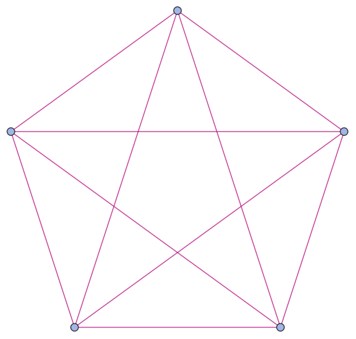
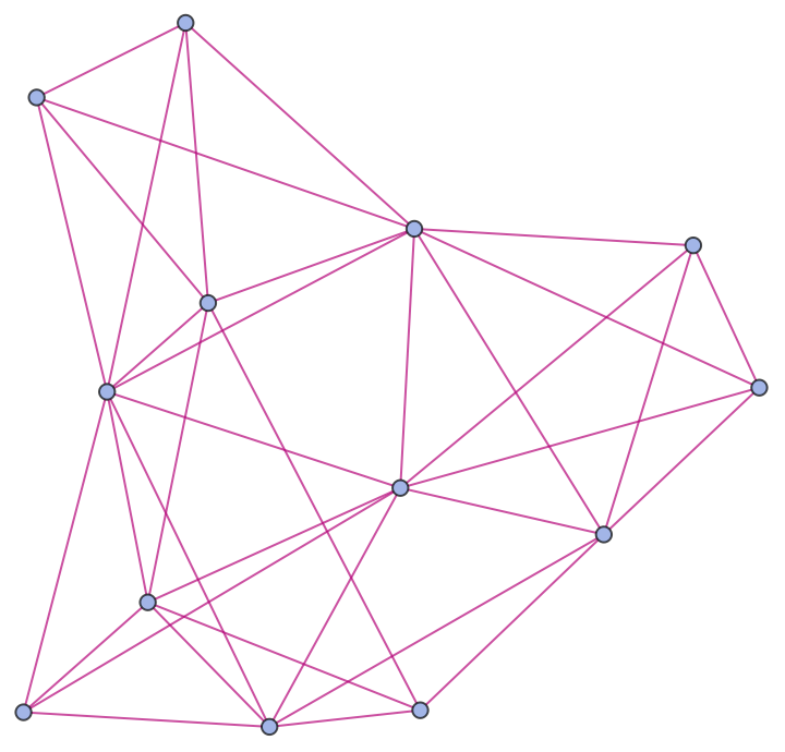
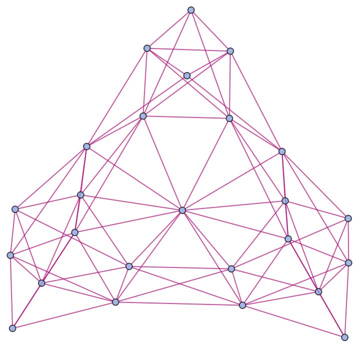
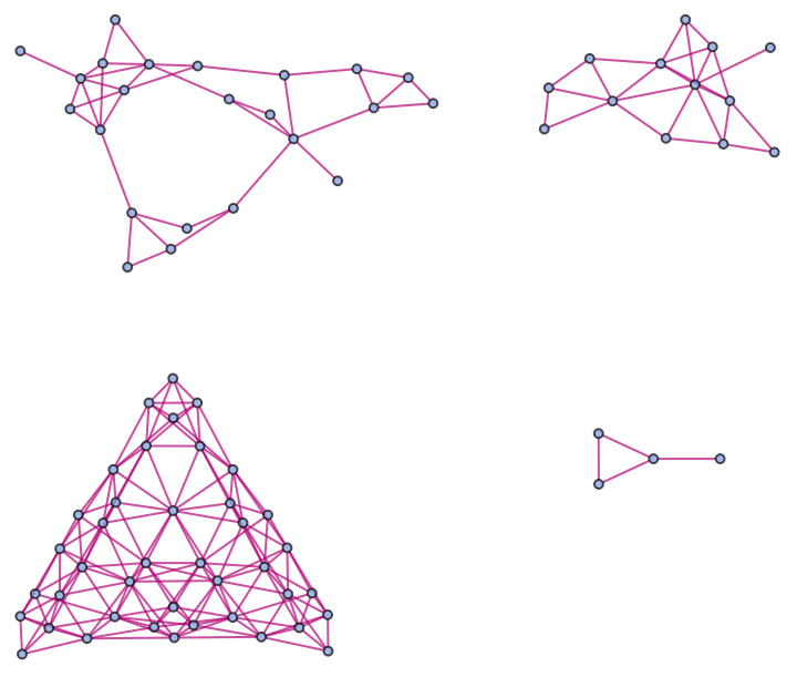
The entropy starts from a minimal value and monotonically increases, eventually flattening out for larger time steps. The corresponding evolution branchial graphs look like:
In[]:=
Table[ResourceFunction["MultiwaySystem"][{"A""ABA","AA""B"},"AABAA",t,"EvolutionBranchialGraphStructure"],{t,6}]
Out[]=
,
,
,
,
,
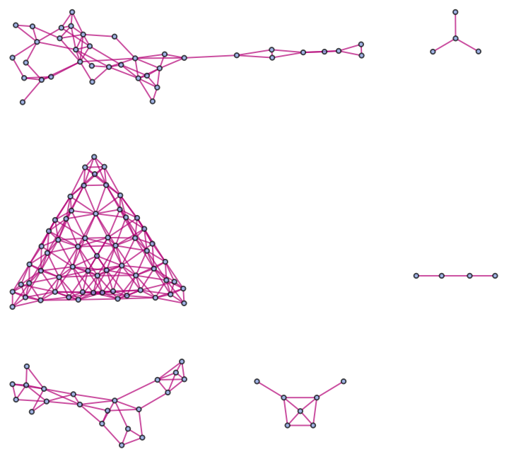
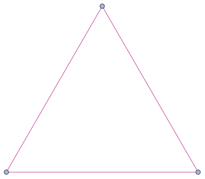
For any complete graph, such as the graph, K_ 5, shown above, the global von Neumann entropy will be equal to zero. Thus, such a branchial graph represents a pure state. All following states increase in entropy. From the above evolution branchial graphs, we observe a splitting of branchial space. However, we compute the combined entropy for all of these states by calculating the complete adjacency matrix’s total density matrix. However, it might be insightful to consider individual, collective states’ entropies to investigate the nature of entanglement horizons.
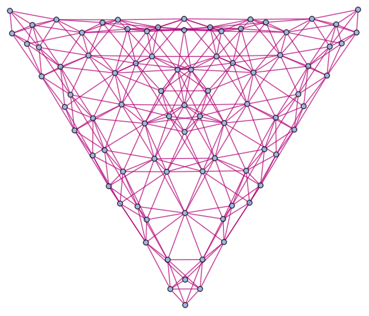
It would be interesting and directly relevant in exploring the Bekenstein bound to compute for more time steps and see whether the entropy approaches some limiting value; however, the current computational cost is too high. Here is another example for the rule “A”->”AB”,”B”->”A” starting from “A”:
It would be interesting and directly relevant in exploring the Bekenstein bound to compute for more time steps and see whether the entropy approaches some limiting value; however, the current computational cost is too high. Here is another example for the rule “A”->”AB”,”B”->”A” starting from “A”:
In[]:=
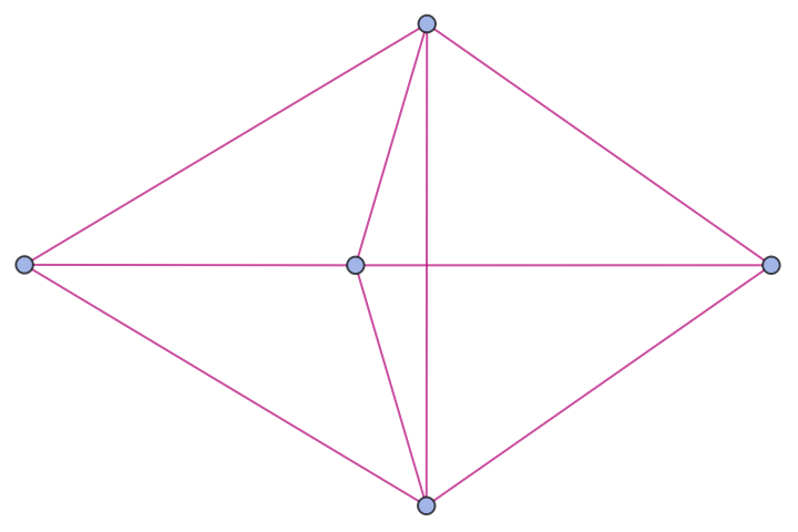
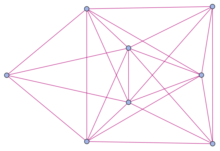
Table[ResourceFunction["MultiwaySystem"][{"A""AB","B""A"},"A",t,"BranchialGraphStructure"],{t,2,7}]
Out[]=
,

,
,
,
,
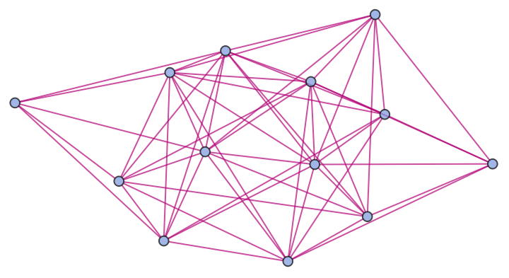
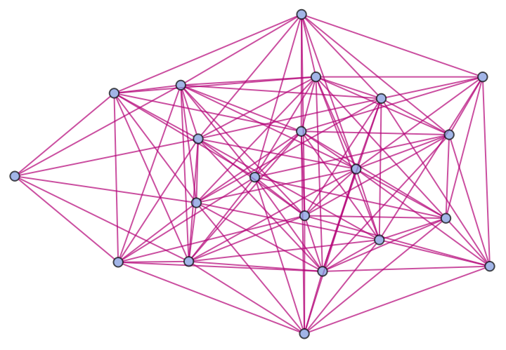
In this case, the entropy increases as follows:
In[]:=
ListLinePlot[GlobalEntropy[{"A""AB","B""A"},"A",7]]
Out[]=
In all considered cases, the initial entropy has minimal value as the system’s initial state corresponds to a pure, maximally connected state. Further exploration of this phenomenon may lead to new insights about the arrow of time and will be part of future investigations.
We note that the entropy’s exact simplified form takes on a very suggestive form for specific density matrices. For example, consider the following density matrix for a three-state system:
Out[]//MatrixForm=
2 | 2 | 2 |
2 | 1 | 1 |
2 | 1 | 1 |
with an adjacency graph:
In[]:=
AdjacencyGraph[p]
Out[]=
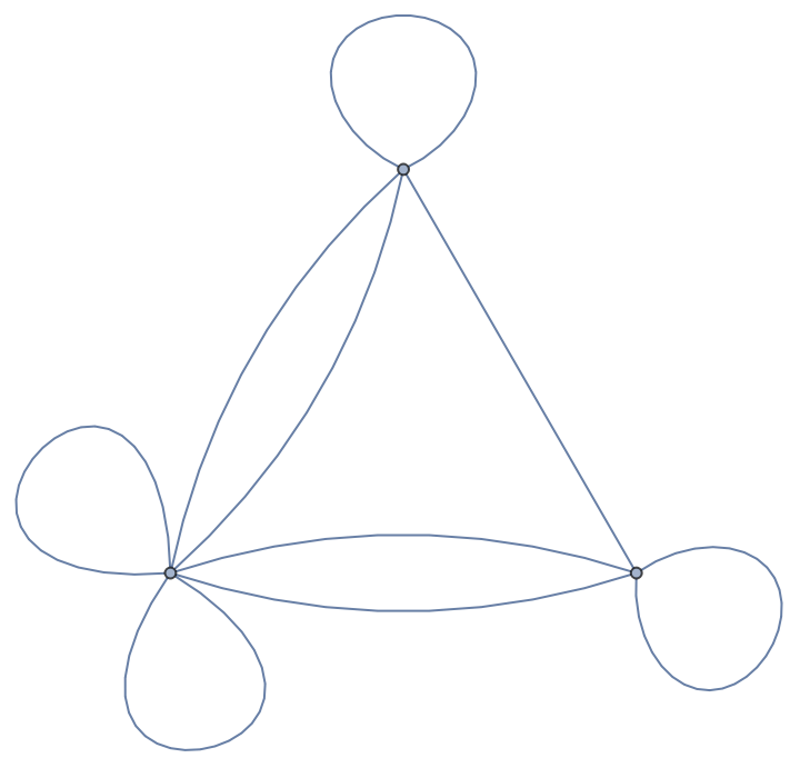
in which the number of edges corresponds to the product of vertex weights of neighboring states and self edges correspond to the individual vertex weights. In this case, the entropy can be written in the form:
If there are n equally likely non-entangled states, there will be n microstates expressed by the Log[n] term. In this case, we note the existence of an additional geometric term plus a phase. This geometric term occurs whenever eigenvalues of the density matrix have a specific form such as:
in this case.
We are particularly interested in exploring this connection to hyperbolic geometry within the context of AdS/CFT.
Local Entanglement Entropy
Local Entanglement Entropy
We can now also trace out a particular subspace of the branchial graph. For example, consider the state “AB” and let us define two regions of that state such that the state can be split up into these two regions as “A” and “B”. Our goal is now to trace out the subsystem corresponding to the second character i.e. region 2. This is illustrated in the example below:
After this, we then compute the von Neumann entropy of the remaining region "A". This entropy provides a measure of the entanglement between the two subsystems. The higher the entanglement entropy, the more information is lost in tracing out a given subsystem. If the local entanglement entropy is zero, there is no entanglement between the two subsystems and we can consider them to be distinct microstates of the global state.
However, this approach will give us an absolute value of local entanglement entropy. In contrast, the microscopic derivation of the Bekenstein Bound requires a relative measure of entropy. Thus, we also need to define the notion of a localized vacuum state, which will be investigated in future work.
Positivity of Relative Entropy
Positivity of Relative Entropy
Having now defined how to derive the local density matrix of a given branchial graph and assuming we have a way to distinguish the vacuum from the excited state, we can compute the Bekenstein Bound by identifying it as the “statement of the positivity of relative entropy between the local density matrices corresponding to the systems state and the vacuum” within a given region [4]. This statement is directly related to the existence of a Fisher information metric describing the geometry of branchial space as was pointed out by Gorard [5].
Thus we can explicitly calculate whether our models satisfy the Bekenstein Bound and in which cases the Bekenstein Bound is saturated. By investigating regions of systems in which the bound is saturated, we can then hope to make direct observations relevant to AdS/CFT.
Connections to AdS/CFT
Connections to AdS/CFT
To make connections with AdS/CFT, we must also understand what holographic surfaces may look like in our models and learn how to compute their areas. Such an understanding will likely emerge by studying various event horizons within Wolfram models and will be part of future investigations. We hope that once the necessary tools and concepts for analyzing the Bekenstein Bound within Wolfram models have been developed and understood, we can make explicit calculations that may demonstrate the AdS/CFT correspondence and gain a more intuitive understanding.
Conclusions
Conclusions
This project has defined concepts relevant to the AdS/CFT correspondence and translated them into Wolfram model terminology. We have identified lacking concepts and tools within the Wolfram model required to make connections to AdS/CFT. One such concept is a global and local notion of entanglement entropy, which we have subsequently defined and computed in string substitution systems by proposing a way to translate branchial space into a density matrix and subsequently trace out a particular subsystem.
Future Work
Future Work
◼
Investigate how to define the density matrix of the vacuum state
◼
Generalize concepts defined in string substitution systems to hypergraph models
◼
Identify systems satisfying the Bekenstein Bound
◼
Classify the nature of holographic surfaces within Wolfram models and calculate their areas.
◼
Concretely relate the tools and findings made to the AdS/CFT correspondence
◼
Investigate the origin of holographic gravity by relating it to causal invariance using the tools we have built.
References
References
◼
Bekenstein, Jacob D. “Black Holes and Entropy.” Physical Review D 7, no. 8 (April 15, 1973): 2333–46. https://doi.org/10.1103/PhysRevD.7.2333.
◼
Ryu, Shinsei, and Tadashi Takayanagi. "Holographic Derivation of Entanglement Entropy from AdS/CFT." Physical Review Letters 96, no. 18 (May 9, 2006): 181602. https://doi.org/10.1103/PhysRevLett.96.181602.
◼
Bousso, Raphael. “Holography in General Space-Times.” Journal of High Energy Physics 1999, no. 06 (June 28, 1999): 028–028. https://doi.org/10.1088/1126-6708/1999/06/028.
◼
Casini, H. “Relative Entropy and the Bekenstein Bound.” Classical and Quantum Gravity 25, no. 20 (October 21, 2008): 205021. https://doi.org/10.1088/0264-9381/25/20/205021.
◼
Gorard, Jonathan. “Some Quantum Mechanical Properties of the Wolfram Model,” n.d., 65.
———. “Some Relativistic and Gravitational Properties of the Wolfram Model,” n.d., 59.
———. “Some Relativistic and Gravitational Properties of the Wolfram Model,” n.d., 59.