ABSTRACT (original article): Motivated by quantum field theory (QFT) considerations, we present new representations of the Euler-Beta function and tree-level string theory amplitudes using a new two-channel, local, crossing symmetric dispersion relation. Unlike standard series representations, the new ones are analytic everywhere except at the poles, sum over poles in all channels, and include contact interactions, in the spirit of QFT. This enables us to consider mass-level truncation, which preserves all the features of the original amplitudes. By starting with such expansions for generalized Euler-Beta functions and demanding QFT-like features, we single out the open superstring amplitude. We demonstrate the difficulty in deforming away from the string amplitude and show that a class of such deformations can be potentially interesting when there is level truncation. Our considerations also lead to new QFT-inspired, parametric representations of the Zeta function and 𝜋, which show fast convergence. CITATION (original article): Arnab Priya Saha and Aninda Sinha (2024), Field Theory Expansions of String Theory Amplitudes, Phys. Rev. Lett. 132, 221601. https://doi.org/10.1103/PhysRevLett.132.221601
From 15th century Madhava to 20th century Feynman: stringing Pi, Aninda Sinha, ICTS News, Volume x, Issue 1, 2024
From 15th century Madhava to 20th century Feynman: stringing Pi, Aninda Sinha, ICTS News, Volume x, Issue 1, 2024
In[]:=
N[Pi,25]
Out[]=
3.141592653589793238462643
The oldest series representation of pi was given to us by the famous Indian mathematician, Madhava in the 14th or 15th century, before the invention of calculus [1] and the incredible book “Series and products in the development of Mathematics” [2]. Madhava’s series for pi (historically referred to as the Madhava-Leibniz series as it was rediscovered by Leibniz in the 17th century) takes the form:

This form of the series converges very slowly to the actual value.
Imagine we are trying to measure the probability of scattering, but we are limited by how much energy we can pump into our experiments. Thus, we cannot excite a very highly massive virtual particle as it would need energies beyond what we have access to. What is the best possible way to describe the physics in such an experiment? The parametric formulas found in this paper enable a quantitative answer to such a question. The explicit formula that emerges for the open superstring amplitude is [3]:The presence of the parameter lambda (denoted by the Greek symbol) in the series is vital. It enables us to interpolate between various physical pictures. For instance, when lambda is set equal to we have an expansion in terms of the singularities in only. Namely we have:

-
s
2
s
1

As physics undergraduates, we learn that the square-root of pi emerges from the Gamma function evaluated at the argument ½. Then from the formula above, getting a formula for pi is literally child’s play! We just set and to be – ½ . Then we have our new formula for π:
s
1
s
2

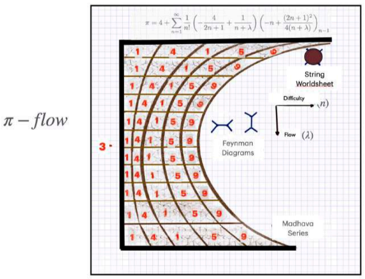
The state of affairs can be explained in the figure for pi below. On the horizontal axis, we depict the number of terms in the series — the larger the number of terms we use, the harder it is to compute. The vertical axis represents the extra physics inspired parameter that was described above. As we dial the parameter, in the middle of the figure, the number of terms needed and hence the difficulty minimizes. As the parameter becomes large, we get the century Madhava series (using which calculating π is a very hard task as an answer to 10 decimal places needs 5 billion terms). As the parameter becomes small, we get a description in terms of the traditional string picture. However, the most efficient is in terms of Feynman diagrams, which is what the middle of the figure conveys (10 decimal places needs around 40 terms)! Our objective was not to find the fastest converging representation! There are many known series representations which converge very fast.
th
15
representation
Playing with the series on Mathematica is fun and addictive—we give sample outputs below. Let’s define truncated version of this formula as a function nMax terms:
piTrunc[λ_,nMax_]:=4+-Pochhammer-n,n-1
nMax
∑
n=1
1
n!
1
n+λ
4
2n+1
2
(2n+1)
4(n+λ)
Grid[Table[{Row[{"λ=",λ}],N[piTrunc[λ,100],50]},{λ,10,100,10}],Dividers->Center]
Out[]=
λ=10 | 3.1415926535897932311167982568600954667218526005880 |
λ=20 | 3.1415926535897932384626436755414307255483599616664 |
λ=30 | 3.1415926535897932384626433831439224135176241204867 |
λ=40 | 3.1415926535897932384626433832794435821686592564136 |
λ=50 | 3.1415926535897932384626433832795014802072032927157 |
λ=60 | 3.1415926535897932384626433832795030581956089721076 |
λ=70 | 3.1415926535897932384626433832795028638105817719887 |
λ=80 | 3.1415926535897932384626433832795028676400412039044 |
λ=90 | 3.1415926535897932384626433832795028933864455844140 |
λ=100 | 3.1415926535897932384626433832795028881249629463115 |
Grid[Table[{Row[{"λ=",λ+I}],N[piTrunc[λ,100],50]},{λ,10,100,10}],Dividers->Center]
Out[]=
λ=10+ | 3.1415926535897932311167982568600954667218526005880 |
λ=20+ | 3.1415926535897932384626436755414307255483599616664 |
λ=30+ | 3.1415926535897932384626433831439224135176241204867 |
λ=40+ | 3.1415926535897932384626433832794435821686592564136 |
λ=50+ | 3.1415926535897932384626433832795014802072032927157 |
λ=60+ | 3.1415926535897932384626433832795030581956089721076 |
λ=70+ | 3.1415926535897932384626433832795028638105817719887 |
λ=80+ | 3.1415926535897932384626433832795028676400412039044 |
λ=90+ | 3.1415926535897932384626433832795028933864455844140 |
λ=100+ | 3.1415926535897932384626433832795028881249629463115 |
The physics considerations provide the motivation for looking for such parametric representations in the first place. More importantly, this picture enables us to think about ways to retain some of the nice features of string theory (it is after all a consistent theory of quantum gravity) while abandoning some of the unwanted ones (e.g. exponential softness in amplitudes). In particular, it will enable a re-examination of some of the roots of string theory and either establish them as the unique direction forward or enable a search for a new realistic perspective of nature.
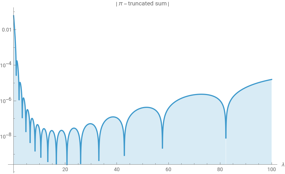
The terms behave asymptotically as:
-
-2-λ
k
Gamma[1-λ]
This means that for integer λ they become small and the convergence is truncation dependent and lambda-dependent:
In[]:=
Manipulate[LogPlot[Evaluate[Abs[Pi-piTrunc[λ,n]]],{λ,0,100},PlotRange->All,WorkingPrecision->100,PlotPoints->100,PlotLabel->Abs[Pi-"truncated sum"],AxesLabel->{"λ",None},Filling->Bottom,ImageSize->500],{{n,16,"terms"},1,50,1,Appearance->"Labeled"}]
Out[]=


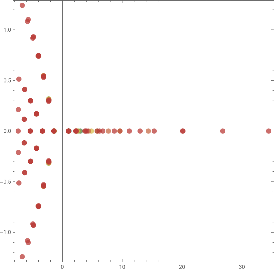
And for each fixed truncation after n terms, there are n (n+1)/2 values of lambda such that the formula becomes ‘exact’:
In[]:=
Graphics[Table[{ColorData["DarkRainbow"][n/6],PointSize[.02],Opacity[.75],Point[ReIm[N[N[SolveValues[piTrunc[λ,n]==Pi,λ],100]]]]},{n,1,8}],PlotRange->All,AspectRatio->1,Axes->True,Frame->True]
Out[]=
Define the absolute value of the difference with π:
Show the convergence over the complex λ plane:
References
References
[2] Ranjan Roy, “Series and products in the development of Mathematics”, Cambridge University Press, 2021.
[3] Arnab P. Saha, Aninda Sinha, “Field Theory expansions of string theory amplitudes,” Physical Review Letters 132 (2024) 22, 221601.
CITE THIS NOTEBOOK
CITE THIS NOTEBOOK
From 15th century Madhava to 20th century Feynman: stringing Pi
by Arnab Priya Saha and Aninda Sinha
Wolfram Community, STAFF PICKS, August 28, 2024
https://community.wolfram.com/groups/-/m/t/3259819
by Arnab Priya Saha and Aninda Sinha
Wolfram Community, STAFF PICKS, August 28, 2024
https://community.wolfram.com/groups/-/m/t/3259819