Wolfram Cloud Document

This post is inspired by the Mathematica StackExchange question which, again, was based on a X/Twitter post. Although these plots involve “insects”, it’s really all about suitable randomness and human visual interpretation of it. A suitably continuous function with random parameters is being sampled; in my case it’s four-dimensional but technically one dimension for individual paths and two dimensions for multiple paths (represented below as different hues) would be sufficient; I just wanted to pedagogically separate the function being sampled and the effects of the range on it which gets sampled. One could also shift the sampled region around and vary the results slightly which wouldn’t be possible in the same way if the whole periodic function range would be sampled for each plot.

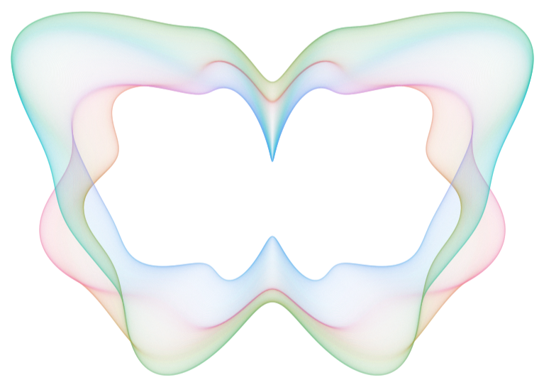
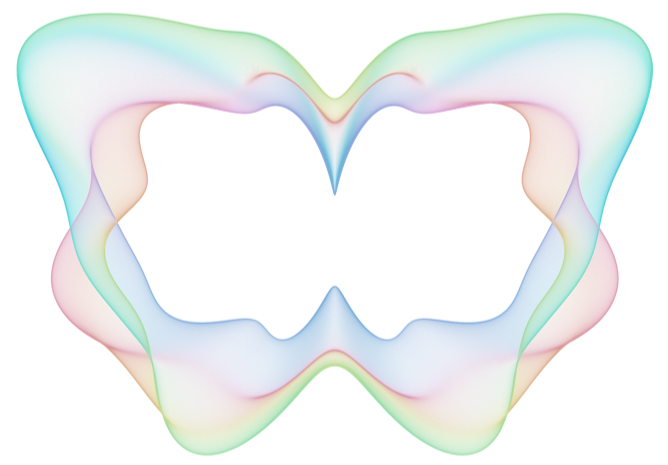
Most animals in nature exhibit bilateral symmetry. The plotted data can be made symmetric along one axis by many ways, and here it’s just about summing values of the above function mirrored along the y axis. This, like Rorschach ink blots, springs human imagination into life and many of the plots resulting from purely random data resemble some sorts of creatures - often insects or bugs - as a result.

Seed for randomness in “noise”

seed=54;

Distance range from the origin

range={1,15};

Points along the a and z directions

na=1000;nz=500;

Raster size for later renderings

rastersize=2000;

Number of frequency terms per dimension

terms=6;

Basis for scaling down higher frequencies

basis=1.3;

Four - dimensional “noise” function - close - by coordinates have more similar values than far away

SeedRandom[seed];noise=Compile[{{x,_Real},{y,_Real},{z1,_Real},{z2,_Real}},(*essentiallyamixofrandomsinewavesinfourdimensions*)Evaluate[Sum[(basis^-(i+j+k+l))RandomReal[{-1,1}]Sin[Pi(ix+RandomReal[{-1,1}])]Sin[Pi(jy+RandomReal[{-1,1}])]Sin[Pi(kz1+RandomReal[{-1,1}])]Sin[Pi(lz2+RandomReal[{-1,1}])],{i,0,terms},{j,0,terms},{k,0,terms},{l,0,terms}]]];

A list of distances from origin for every color

distances=ParallelTable[Table[With[{(*xandyaretheregularvaluesalongthecircle*)x=Sin[a],y=Cos[a],(*z1andz2arevaluesaroundthetwootherdimensions,fordifferentcolors*)z1=Sin[z],z2=Cos[z]},(*summingmirroredversionsmaketheresultsymmetricalongxaxis*)noise[x/2,y/2,z1/10,z2/10]+noise[-x/2,y/2,z1/10,z2/10]],{a,0.,2Pi,2Pi/na}],{z,0.,2Pi(1-1/nz),2Pi/nz},Method->"CoarsestGrained"]//(*onceadistancelistforeverycolorhasbeencomputedscaleallofthemontherange*)Rescale[#,MinMax[Flatten[#,1]],range]&;

Corresponding points on the unit circle

circlepoints=Table[{Sin[a],Cos[a]},{a,0.,2Pi,2Pi/na}];

Colors for every distance list

colors=Table[LABColor[0.7,0.41Sin[h],0.41Cos[h]],{h,0,2Pi(1-1/nz),2Pi/nz}];

Actual point lists in the {x, y} form, scaling circlepoints with distances

points=MapThread[#1#2&,{circlepoints,#}]&/@distances;

Separate lines for graphics

lines=Line/@points;

Actually plot a bug

Graphics[{(*draweverythingwiththinsemi-transparentlines*)Thin,Opacity[1/4],(*littletweaksonrendering*)CapForm[None],JoinForm[None],(*everylinewithitscolor*)Transpose[{colors,lines}]},ImageSize->Large]

Out[]=

Compute coordinate bounds for image stacking

bounds=CoordinateBounds[Flatten[points,1],Scaled[0.025]];

Compute maximum brightness across a stacked image

brightness=Fold[ImageAdd[#1,Image[Rasterize[Graphics[{White,Thin,CapForm[None],JoinForm[None],#2},Background->Black,PlotRange->bounds],RasterSize->rastersize],"Real"]]&,(*real-valuedblackstartingimage*)Image[Rasterize[Graphics[Background->Black,PlotRange->bounds],RasterSize->rastersize],"Real"],lines];

Stack colored lines, each on separate image

hues=Fold[(*addanimagewithonecolortotheprevious*)ImageAdd[#1,Image[Rasterize[Graphics[{Thin,CapForm[None],JoinForm[None],#2},Background->Black,PlotRange->bounds],RasterSize->rastersize],"Real"]]&,Image[Rasterize[Graphics[Background->Black,PlotRange->bounds],RasterSize->rastersize],"Real"],Transpose[{colors,lines}]];

(*dosomead-hoccompositionmagicwithhuesandbrightnesses-withalphachannel*)alphaimage=ColorSeparate[ColorConvert[hues/Max[brightness],"HSB"]]//ColorCombine[{#[[1]],0.8#[[2]],ConstantImage[0.85,ImageDimensions[hues]],ColorConvert[brightness/Sqrt[Max[brightness]],"Grayscale"]^(1/1.5)},"HSB"]&//(*convertintoaregular8-bitRGBAimage*)Image[ColorConvert[#,"RGB"],"Byte"]&

Out[]=

With black background

Seed 56

Seed 60

Seed 62

Seed 64

Seed 80

Seed 84

Seed 86

Seed 87

Seed 91

Seed 98

Seed 102

CITE THIS NOTEBOOK

Insect-shaped mandalas: 4D noise mapped to 2D distance-based color and line generation
by Jari Kirma
Wolfram Community, STAFF PICKS, January 28, 2025
https://community.wolfram.com/groups/-/m/t/3366045