Hey all, I recently read through the Wikipedia page on the Cahn-Hilliard equation, which is used to model phase separation/spinodal decomposition, and I thought I’d implement it in Mathematica. The results are OK, plenty of room for improvement, but it’s worth sharing!
The Cahn-Hilliard equation is an interesting nonlinear partial differential equation which can be used to model spinodal decomposition (two phases rapidly settling out). It’s quite nonlinear, so let’s see how NDSolve handles it!
In[]:=
TraditionalForm[Hold[Derivative[0,0,1][c][x,y,t]==dLaplacian[c[x,y,t]^3-c[x,y,t]-γLaplacian[c[x,y,t],{x,y}],{x,y}]]]
Out[]//TraditionalForm=
Hold(x,y,t)d-c(x,y,t)-γc(x,y,t)
(0,0,1)
c
2
∇
{x,y}
3
c(x,y,t)
2
∇
{x,y}
Initial Conditions
Initial Conditions
First, we create an interpolating function for the initial condition:
In[]:=
Clear[grid0];gridn=50;gridm=50;grid0[i_,j_]:=grid0[i,j]=RandomReal[{-4,4}];mean=Sum[grid0[i,j],{i,1,gridn},{j,1,gridm}]/(gridngridm);grid[i_,j_]:=grid0[i,j]-mean;dx=1/(gridn+1);dy=1/(gridm+1);initialc=Interpolation[Flatten[Table[{{dxi,dyj},If[i==0||j==0||i==gridn+1||j==gridm+1,0,grid[i,j]]},{i,0,gridn+1},{j,0,gridm+1}],1]];
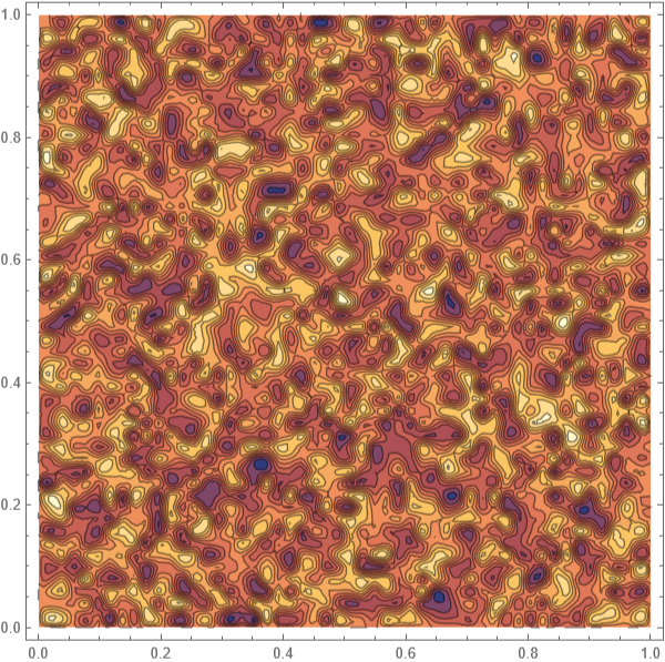
We get a nice noisy interpolated function for the initial condition:
In[]:=
ContourPlot[initialc[x,y],{x,0,1},{y,0,1}]
Out[]=
Solving the PDE
Solving the PDE
Solve the Cahn-Hilliard equation. Compare to https://en.wikipedia.org/wiki/Cahn%E2%80%93Hilliard_equation#/media/File:CahnHilliard_g0.5.gif
◼
I didn’t yet have the patience to increase the number of grid points, maybe adding the option to NDSolve Method {“MethodOfLines”, “SpatialDiscretization” {“TensorProductGrid”, MaxPoints 500}}
◼
In the image on wikipedia, the domain goes from -40 to 40 with D=1 and gamma=0.5. So, a quick analysis of units says that to reproduce that image with our domain going from 0 to 1, we should have D=1/80^2 and gamma=0.5/80^2. I can’t go quite so extreme with the default number of grid points, but that’s why the coefficients are taken to be so small.
In[]:=
diff=1/30.0^2;gamma=0.5/30.0^2;eoms={c[x,y,0]==initialc[x,y],c[0,y,t]==c[1,y,t],c[x,0,t]==c[x,1,t],Derivative[0,0,1][c][x,y,t]==diffLaplacian[c[x,y,t]^3-c[x,y,t]-gammaLaplacian[c[x,y,t],{x,y}],{x,y}]};csoln=NDSolveValue[eoms,c,{x,0,1},{y,0,1},{t,0,5}]
We see we get the expected somewhat flat regions of concentration +1 and -1.
In[]:=
Plot3D[csoln[x,y,5.0],{x,0,1},{y,0,1}]
Out[]=

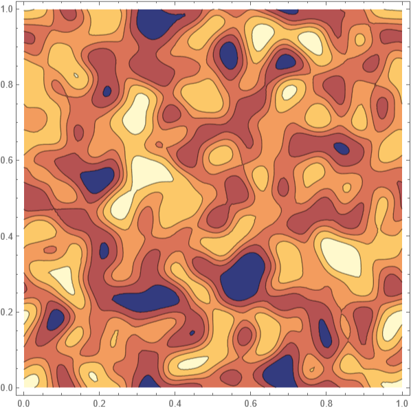
A contour plot as the phases are just starting to separate:
In[]:=
ContourPlot[csoln[x,y,0.1],{x,0,1},{y,0,1}]
Out[]=
Exporting a video
Exporting a video
Plotting the evolution in a 240 frame 30 fps video:
In[]:=
nframes=240;frames=Table[DensityPlot[csoln[x,y,t],{x,0,1},{y,0,1},ColorFunction->(ColorData["TemperatureMap"][(#+1)/2]&),ColorFunctionScaling->False],{t,0,5,5/240}];Parallelize@FrameListVideo[frames,RasterSize->480,FrameRate->30]
Out[]=
CITE THIS NOTEBOOK
CITE THIS NOTEBOOK
Example of solving the Cahn-Hilliard equation with NDSolve
by David Moore
Wolfram Community, STAFF PICKS, October 6, 2024
https://community.wolfram.com/groups/-/m/t/3291843
by David Moore
Wolfram Community, STAFF PICKS, October 6, 2024
https://community.wolfram.com/groups/-/m/t/3291843