Protein folding algorithms play a crucial role in protein research by organizing data efficiently and facilitating insights into molecular structures. These algorithms navigate complex processes, considering residue traits and other factors to accurately predict protein structures. This project aims to analyze the distribution of structural parameters derived from randomly generated amino acid sequences. By generating 1000 proteins with a sequence length of 100 amino acids, employing diverse characterization methods, and conducting thorough data analysis, this study seeks to uncover patterns and distributions that illuminate the underlying principles of protein folding.
Introduction
Introduction
With the rise of protein folders, there is an increasing interest on the functionality of how protein folders work. Protein folders take in a linear amino acid sequence then generate an estimated 3D structure corresponding to the many factors and traits of the residues (or amino acids). ESM is a protein folder with a great level of complexity that works quickly and accurately to predict the structure of the generated sequence. My project analyzes the distribution of shape parameters produced by the protein folder. With this analysis, there is a better understanding on how ESM fold generally works and patterns that shape the accuracy of the predictions. This understanding could potentially lead to advancements in protein structure prediction and contribute significantly to fields such as drug discovery and molecular biology. By delving into the traits of protein folding shape outputs, this study aims to uncover insights that enhance our comprehension of biological processes at the molecular level.
Shape Parameters Data Set
Shape Parameters Data Set
With the 1000 random amino acid sequence folds, I created shape characteristics and stored them into lists to use for graph analysis.
In[]:=
shapeInfo = ;dimensionsInfo = ;tailDistanceInfo = ;stretchedDistanceInfo = ;convexVolumeInfo = ;concaveVolumeInfo = ;atomBoxVolumeInfo = ;convexBoundaryVolumeInfo = ;concaveConvexVolumeInfo = ;percentEmptyVolumeInfo = ;bigHolesInfo = ;convexDensityInfo = ;concaveDensityInfo = ;boxesDensityInfo = ;
Importing and Basic Functions
Importing and Basic Functions
Mathematica 14.0 has a built in ESM folder function to generate a protein structure, but this structure only contains the back bone of the protein. This means that other atoms such as the side chains and more would be ignored for the structuring and shape parameters. To work around this issue, I downloaded an early access paclet from Mathematica 14.1. This paclet provided a variety of traits in the structure of a protein such as most atom coordinates excluding hydrogens, residues, and residue roles. I also created a graphics3D function to ensure that all generated structures/bounds would face the same direction and contain the same ground parameters.
In[]:=
PacletInstall["WolframChemistry/ProteinVisualization"];Needs["WolframChemistry`ProteinVisualization`"];PDBImportDataFromBioSequence[bs_BioSequence]:=Replace[WolframChemistry`ProteinVisualization`Private`proteinStructure[bs],WolframChemistry`ProteinVisualization`Private`proteinStructure[a_Association]:>a]graphics3D[graphics_]:=Graphics3D[graphics,ViewPoint->Above,Boxed->True,Axes->True,ViewVertical->{0,0,1}]
Generating Random Amino Acid Sequences and 3D Points of Structure
Generating Random Amino Acid Sequences and 3D Points of Structure
In this section, I generated random 100 length amino acid sequence with equal probabilities to the corresponding residues. For my data analysis I generated 1000 proteins for a good variety of data. Since I had to create many proteins at once, I used numberOfProteinsToGenerate in order to run multiple random amino acid sequences. With these sequences, I called the 14.1 paclet folder to create a list of associations for data points.
In[]:=
numberOfAA=100;(*lengthofrandomaminoacidsequence*)aminoAcids={"A","R","N","D","C","Q","E","G","H","I","L","K","M","F","P","S","T","W","Y","V"};probability={3,3,3,3,3,3,3,3,3,3,3,3,3,3,3,3,3,3,3,3};normalizedProbability=probability/Total[probability];numberOfProteinsToGenerate=1;randomAminoAcids:=StringJoin[RandomChoice[normalizedProbability->aminoAcids,numberOfAA]];generatedAminoAcids=Table[randomAminoAcids,numberOfProteinsToGenerate];collectiveAllPoints=PDBImportDataFromBioSequence[BioSequence["Peptide",#]]&/@generatedAminoAcids;
Here is an example of the associations the call to the 14.1 folding paclet returns with the different residues, atoms, and atom locations.
Out[]=
How Results Are Set Up
How Results Are Set Up
Below every graph, visualization, or display, I explain the results and conclusion of the data. Under the explanation I included the code that generated the data to create those displays. There may also be examples of certain points on the displayed graph. If you would like to run this notebook, this does not run on wolfram cloud but works when downloaded into a file do to the properties of using a 14.1 paclet.
Best Fitting Shape
Best Fitting Shape
To characterize the general shape that could best capsulate all the points, I used BoundingRegion and found the “best shape” by taking the shape with the least volume. Within the variety of different bounding regions, there were only two best fitting bounding regions types: the MinOrientedCuboid and MinEllipsoid. Within the cuboids, I took the largest diagonal from opposite points and plotted the distribution of their lengths. Within ellipsoids, I took the largest semi-axis and plotted the distribution of their lengths. The cyan colored dots are the backbone of the protein while the dark blue dots represent the other atoms within the structure.
In[]:=
shapeDimensions=Map[bestFittingShape,collectiveAllPoints[[Range[numberOfProteinsToGenerate]]]];

In[]:=
shapeInfoCount=Counts[shapeInfo];BarChart[shapeInfoCount,ChartLabels->Keys[shapeInfoCount],ChartStyle->{Blue,Red},BarSpacing->0.7,Frame->True,FrameStyle->Directive[Black,12],PlotLabel->Style["Distribution of Best Fitting Shapes",Black]]
Out[]=
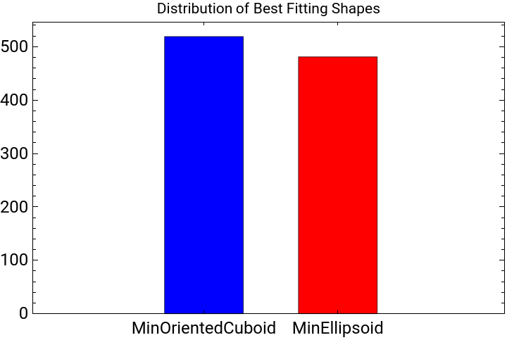
In random amino acid sequences, ESM fold slightly favors MinOrientedCuboid shapes over MinEllipsoids when creating the structures enclosing boundaries.
cuboidShapeDimensions=Select[dimensionsInfo,NumberQ]/100;SmoothHistogram[cuboidShapeDimensions,PlotLabel->Style["Distribution of Cuboid Shape Dimensions",Black],PlotStyle->Directive[Red,Thick],Frame->True,FrameLabel->{"Diagonal Length (Angstroms)","Density"},FrameStyle->Directive[Black,12]]
Out[]=
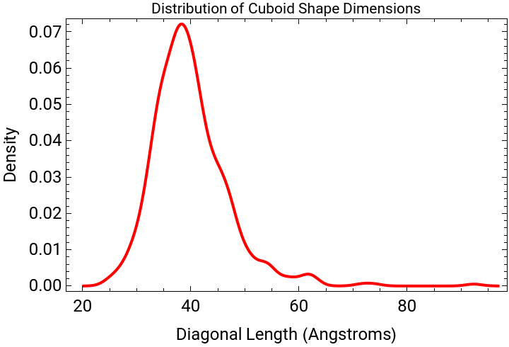
The diagonal length cuboid distribution is slightly skewed towards 40 A . There are some outliers with larger diagonal length then most, which could show how the structure wasn’t able to compact into a ball rather more like an elongated shape, possibly with a tail.
In[]:=
ellipsoidShapeDimensions=ToExpression[Cases[dimensionsInfo,_String]];ellipsoidLargestSemiAxis=Max/@ellipsoidShapeDimensions;SmoothHistogram[ellipsoidLargestSemiAxis,PlotLabel->Style["Distribution of Ellipsoid Shape Dimensions",Black],PlotStyle->Directive[Red,Thick],Frame->True,FrameLabel->{"Largest Semi Axis Length (Picometers)","Density"},FrameStyle->Directive[Black,12]]
Out[]=
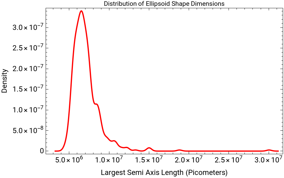
The ellipsoid largest semi axis length also shows a heavily skewed distribution. There are some outliers with larger length then most, which could show how the structure wasn’t able to compact into a ball rather more like an elongated shape, possibly with a tail.
Tail Finder
Tail Finder
Another characteristic of the structures are tails and loops. Usually having a tail/loop shows that the protein either has a very hydrophilic region or end. This parameter causes the structure to be more unraveled and have a greater variation for other parameters as well like volume. During this exploration I created 3 different versions with Tail Finder 3.0 as the quickest and most accurate.
Tail Finder 1.0 (slow and inaccurate)
Tail Finder 1.0 (slow and inaccurate)
In Tail Finder 1.0 I used atom coordinates and their residue number in find clusters to create different groups group. Including amino acid residues as a fourth parameter in FindClusters and using a different methods didn’t cared too much of the impact of amino acid residues. This often caused it to just cut the structure into different sections based of the number of clusters and consecutive amino acid residues. It also took too much time to run through 1000 different samples of randomly generated points so I tried creating another tail finder method.
Tail Finder 2.0 (inaccurate)
Tail Finder 2.0 (inaccurate)
Tail Finder 1.0 was my first method with taking in 4 parameters instead of 3. Tail Finder 2.0 uses 3 parameters and completely ignores amino acid chains. This was inaccurate as it often took points from other points of the structure if it was close to the tail. It sometimes also included multiple parts of the structures such as amino acids from different consecutive residues. This was cleaned up in Tail Finder 3.0.
Tail Finder 3.0
Tail Finder 3.0
With Tail Finder 3.0, I only used the atom coordinates in Find Clusters, took the furthest cluster, grouped it by consecutive amino acids, and removed outliers from the cluster points. I used the distance ratios between the centroids of these clusters to create a “tailness” number to see if the structure contains a tail. During my cluster exploration, I tried many different methods and variations and found that the 3rd version was the most accurate and quickest. In this version of tail finder the red region was the cluster furthest away.
This is a sharply skewed distribution. I speculate that sequences with a “tailness” over 1.6 are much more likely to have a visually apparent tail. This graph shows that ESM fold is likely to fold a compact structure with no tail, while there are some outliers with tails.
Here is an example where the tailness factor was a 1.98806 and generated a structure with a tail colored in red. The amino acid sequence was VMCIRVKDLNIYTWSYIETCSHLWKQNSLEVILHQRITWVFEPRNCFCIEEWHMRPKAIRDSGEPPEDPATACLLKLKRIHKRKSVYKSTRNQKDELKNR and had a very hydrophilic end.
Largest Distance
Largest Distance
Another characteristic for the structures was how much the sequence folded. I calculated the ratio of the distance from the two furthest points from atoms and the stretched out length of the structure. The mean value for most inter-alpha carbon atom bonds is 3.85 Angstroms. I took the total inter-alpha carbon atom distance and took that as the stretched out length of the structure. While there are extra atoms on the ends of the last inter-carbon, the lengths are negligible compared to the total stretched out length. This ratio represents how compact or folded the structure is. The lower the ratio, the more folded the structure is while the higher the ratio the more unraveled it was.
This is a slightly skewed graph of the furthest distance in the actual structure compared to the stretched out structure of the sequence. The ratio of the actual/stretched out distance is almost the same for all 100 length amino acid sequences with a density of 36.1 at 0.1275 ratio.
AA Sequence Traits and Display
AA Sequence Traits and Display
A major contributing part of residue folding are the characteristics of the residues. To help understand these effects, I graphed the the different atoms of the residues and colored them off the traits. Generally, hydrophilic residues (positively/negatively/polar charged) point towards the outside of the structure as they tend to like water (H2O) molecules better. The hydrophobic residues are usually on the inside of the structure and form hydrophobic interactions due to their dislike of water. Another major contributor to the shape of the protein are salt bridges and that are created between positively charged and negatively charged residues to connect different areas of the structure. There are also different important special bonds such as disulfide bonds and hydrogen bonds which contribute to the structures as well.
This display shows the different traits of the amino acid residues. Red represents the positively charged, blue the negatively, green the polar charged, orange the hydrophobic, and special in yellow. It shows the relationships between the residues that cause the structure to fold and have different interesting shapes.
Volume Distributions
Volume Distributions
Another major shape characteristic of the random structures is volume. I had three ways of getting that volume. One was the convexHull volume which was a great overestimate compared to the actual volume of the structure. It included the volumes of the H2O molecules and cavities of the structure causing the volume to be much greater then the actual solvent accessible surface volume of the structure. I also tried concave volume which created a similar structure to the actual fold, but it had poor accuracy. For ConcaveHullMesh, when you pass in a radius it makes the volume thicker and connects to more points. With a super small radius, its almost like connecting the points with thin sheets of volume. While this may work for other structures in the folded proteins, the points are so tightly compacted that increasing the radius would connect them and overestimate the volume. To make it more accurate I picked a radius in between those effects but its still an underestimate compared to the actual volume.
The concave volume differs greatly from the convex and atom box volume. This is most likely because the thickness of the structure is extremely thin, not actually capturing the full volume of the structure.
There was a fourth way to get an estimated volume, with BoundaryRegion but this volume was very inaccurate. The purple line or convex/boundary ratio is much more normally distributed compared to the other ratios, showing there wasn’t any particular strong pattern. The concave/convex and atom box/convex have really similar peaks in density and are slightly skewed.
There is a modest correlation between the convex and atom box volume. There is one obvious outlying point which suggests a correlation too.
ConvexHullMesh Volume
ConvexHullMesh Volume
This generates the ConvexHullMesh Volume and the ratio of the ConvexHullMesh/BoundaryVolume. This is graphed in red above and shows how inaccurate the boundary volume is as it includes a lot of empty space surrounding the folded protein.
ConcaveHullMesh Volume
ConcaveHullMesh Volume
Under you can observe how with the increased radius from 250 -> 400 picometers, ConcaveHullMesh connected many more points and formed an overestimate compared to the actual volume. Below the structures are the corresponding volumes of the meshes. The concave hull mesh with To create a more accurate volume generator, I made my own volume generator located below. After the volumes the function returns the concavehullmesh volume and concavehullmesh/convex volume ratio.
Atom Box/Concavities
Atom Box/Concavities
With ConvexHullMesh volume being an overestimate and ConcaveHullMesh volume being an underestimate, Atom Box volume is like a middle ground with a slight bit of overestimation due to box edges. For a more accurate volume of the structure I decided to use the volumes of small cubes. If the box contained a atom, it would then be counted as a cube of the volume for the structure of the folded protein. Boxes that contain no atoms but are inside the convex hull mesh (to minimize random outer H2O space) are shown with their centers as green dots below. Each cube has a side of 275 picometers or 2.75 angstroms as a water molecule is around 2.75 angstroms of size. While this does not mean that there is one water molecule per dot due to how water can compact, its a good way of showing concavities within the protein.
To display the porousness/concavities, I took all empty cubes within the convex hull that had more then 20 other empty cube neighbors. I then took that number and divided it by the convex volume to show the distribution of concavities in ratio to size.
This concavity parameter appears to be normally distributed.
Below is an example of a structure with many concavities and a empty neighbor space ratio of: 0.00203823
The amino acid sequence is - MKGLYRSYWMWYTYYRNMITYQCAGEKSDKPILHYAPHTAKEFICAISHQDGICDGFSSEHIVKKYIHRQMTRKFCTANTRYYMMAENGFPFNIMFDIVP
The amino acid sequence is - MKGLYRSYWMWYTYYRNMITYQCAGEKSDKPILHYAPHTAKEFICAISHQDGICDGFSSEHIVKKYIHRQMTRKFCTANTRYYMMAENGFPFNIMFDIVP
Density
Density
Another characteristic of these structures are densities. To calculate the densities, I took the masses of all the atoms and divided them by the volume for each of the three different ways I had for finding volumes. While I did not have access to the hydrogen atoms, their masses are negligible in graphing. Below you can see why the concave volume is inaccurate as the difference between the densities is way greater then the other two volume density comparisons.
From the calculations of the volume, this graph is like an inverse of what was presented under the section of volume distributions as density is held constant.
Amino Acid Length
Amino Acid Length
Another major contributing factor to the folding of the amino acid sequences was the length. With a length of 50 amino acids, the structure was much more tail-like and had a unraveled structure. This is most likely due to having such a small number of residues doesn’t give it enough residues to interact with and then fold onto itself. I also observed that as the length of amino acids became greater to 200 and 300, the protein seemed to be more folded, becoming more compact with a longer length of residues. Below I displayed the graphs of some examples of 50, 100, 200, and 300 amino acid sequence lengths.
Conclusion
Conclusion
Through my exploration, I characterized 1000 randomly generated amino acid sequences, analyzing their folds across numerous shape parameters and examining the distributions of each. The conclusions drawn from each parameter are detailed within their respective sections. Notably, the data revealed significant skewness in metrics such as volume, density, and structural tailness. Specifically, structures exhibiting more pronounced tail-like features tended to exhibit larger volumes and lower densities. Some parameters, like concaveHullMesh volume, proved less successful in their predictive capabilities. Moreover, I analyzed the concavities within these structures and explored how various residue traits influence their formation. This exploration sheds light on the effects that amino acid composition can have on protein structure, contributing to a deeper understanding of protein folding dynamics and their implications in biological processes.
Future Directions
Future Directions
Looking ahead, there are numerous areas of improvement and further exploration in my research. Given more time, I would have liked to individually analyze each of the 1000 proteins generated, potentially increasing the dataset size for more robust and accurate results. Additionally, comparing these randomly generated proteins to real proteins would provide valuable insights into the reliability and applicability of the models developed. Exploring how modifications in the probability of amino acids impact shape parameters due to variations in residue polarity is another area of interest. This analysis could reveal correlations between amino acid characteristics and resulting protein structures. In future iterations of this project, I plan to refine the methodology by removing certain shape parameters like concave volume and enhancing tools such as the tail/loop finder and concavity descriptors. These improvements aim to streamline the analysis process and provide clearer insights into protein structure characteristics. Furthermore, investigating the impact of amino acid sequence length on shape parameters is something I would’ve liked to explore. Lastly, I aspire to explore how shape parameters correlate with protein function. This could demonstrate how specific structural characteristics relate to biological functions, potentially uncovering new relationships between protein structure and function.
Acknowledgements
Acknowledgements
I would like to thank Stephen Wolfram and the program directors for establishing the framework for my computational essay and helping create the direction for my project. I would also like to extend my gratitude to my mentor David DeBrota for his endless support and innovation to help extend my project across more parameters. Without him this project would not be possible. Finally, I would like to thank my peers Tony Song and Shivika Gupta for their unending support and help throughout my project.
References
References
◼
1. Cohen, M., Potapov, V., & Schreiber, G. (2009). Four Distances between Pairs of Amino Acids Provide a Precise Description of their Interaction. PLOS Computational Biology/PLoS Computational Biology, 5(8), e1000470–e1000470. https://doi.org/10.1371/journal.pcbi.1000470
◼
2. ESM Metagenomic Atlas | Meta AI. (2024). Retrieved July 11, 2024, from Esmatlas.com website: https://esmatlas.com/resources?action=fold
◼
3. martin chaplin: martin.chaplin@btinternet.com. (2020). Water molecule structure. Retrieved July 11, 2024, from Lsbu.ac.uk website: https://water.lsbu.ac.uk/water/water_molecule.html
◼
4. Mean distance between the α-carbons of each of the 20 disulfide... (2024). Retrieved July 11, 2024, from ResearchGate website: https://www.researchgate.net/figure/Mean-distance-between-the-a-carbons-of-each-of-the-20-disulfide-configurations-in-NMR-and_fig2_6198980
CITE THIS NOTEBOOK
CITE THIS NOTEBOOK
Distributions of shape parameters for randomly generated amino acid sequences
by Annie Zhu
Wolfram Community, STAFF PICKS, July 11, 2024
https://community.wolfram.com/groups/-/m/t/3217184
by Annie Zhu
Wolfram Community, STAFF PICKS, July 11, 2024
https://community.wolfram.com/groups/-/m/t/3217184