Introduction
Introduction
We do not examine the data source and we do not want to reason too much about the data using the stats. We started this notebook by just wanting to make the bubble charts (both 2D and 3D.) Nevertheless, we are tempted to say and justify statements like:
◼
Pareto holds, as usual.
◼
Language creators tend to do it more than once.
◼
Data ingestion
Data ingestion
In[]:=
url="https://pldb.io/posts/age.tsv";dsData=ResourceFunction["ImportCSVToDataset"][url,"Dataset","FieldSeparators"->"\t"];dsData[[1;;4]]
Out[]=

Out[]=

In[]:=
ResourceFunction["RecordsSummary"][dsData,"MaxTallies"->12]
Out[]=
,
,
,
,
,
,
,
,
,
,
,
,
1 id | ||||||||||||||||||||||||
|
2 name | ||||||||||||||||||||||||
|
3 pldbScore | ||||||||||||
|
4 rank | ||||||||||||
|
5 appeared | ||||||||||||
|
6 tags | ||||||||||||||||||||||||
|
7 creators | ||||||||||||||||||||||||
|
8 ageAtCreation | ||||||||||||
|
9 foundationScore | ||||||||||||
|
10 numberOfUsersEstimate | ||||||||||||
|
11 numberOfJobsEstimate | ||||||||||||
|
12 inboundLinksCount | ||||||||||||
|
13 measurements | ||||||||||||
|
Here is a list of languages we use to "get orientated" in the plots below:
In[]:=
lsFocusLangs={"C++","Fortran","Java","Mathematica","Perl 6","Raku","SQL","Wolfram Language"};
Here we find the most important tags (used in the plots below):
In[]:=
lsTopTags=ReverseSortBy[Tally[Normal@dsData[All,"tags"]],Last][[1;;7,1]]
Out[]=
{pl,textMarkup,dataNotation,library,grammarLanguage,stylesheetLanguage,queryLanguage}
Here we add the column "group" based on the focus languages and most important tags:
In[]:=
dsData=dsData[All,Append[#,"group"->Which[MemberQ[lsFocusLangs,#name],"focus",MemberQ[lsTopTags,#tags],#tags,True,"other"]]&];
Here are dataset’s dimensions (at this point):
In[]:=
Dimensions[dsData]
Out[]=
{215,14}
Distributions
Distributions
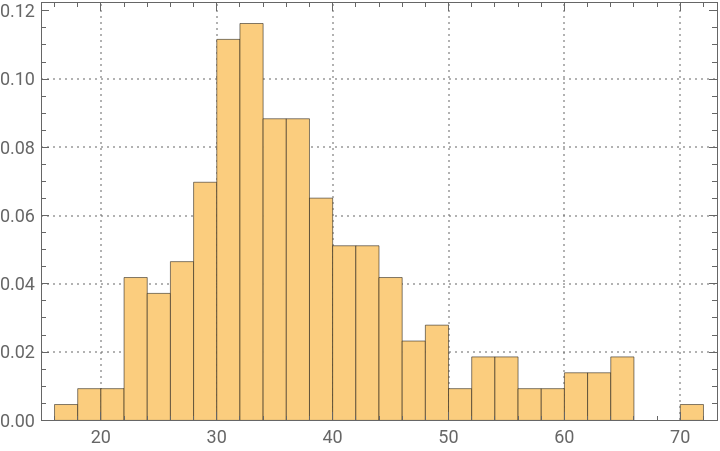
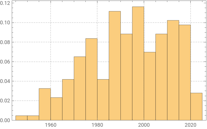
Here are the distributions of the variables/columns:
◼
age at creation
◼
i.e. "How old was the creator?"
◼
appeared"
◼
i.e. "In what year the programming language was proclaimed?"
In[]:=
Association@Map#->HistogramNormal@dsData[All,#],20,"Probability",&,{"ageAtCreation","appeared"}
Out[]=
ageAtCreation
,appeared
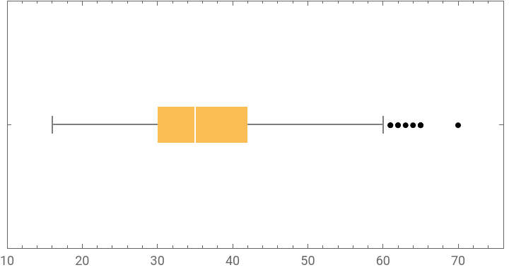
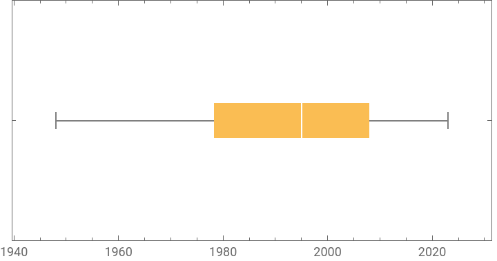
Here are corresponding Box-Whisker plots together with tables of their statistics:
In[]:=
aBWCs=Association@Map#->BoxWhiskerChartNormal@dsData[All,#],"Outliers",&,{"ageAtCreation","appeared"};aBWCs=AssociationThread[Keys[aBWCs],Transpose[{Values[aBWCs],#[[2]]&/@Cases[aBWCs,Tooltip[___],∞]}]]
Out[]=
ageAtCreation
,appeared
,
max | 70 |
75% | 42 |
median | 35 |
25% | 30 |
min | 16 |
,
max | 2023 |
75% | 2008 |
median | 1995 |
25% | 7913 4 |
min | 1948 |
Pareto principle manifestation
Pareto principle manifestation
Number of creations
Number of creations
Here is the Pareto principle plot of for the number of created (or renamed) programming languages per creator (using the WFR function ParetoPrinciplePlot):
In[]:=
ResourceFunction["ParetoPrinciplePlot"][Association[Rule@@@Tally[Normal@dsData[All,"creators"]]],ImageSize->Large]
Out[]=
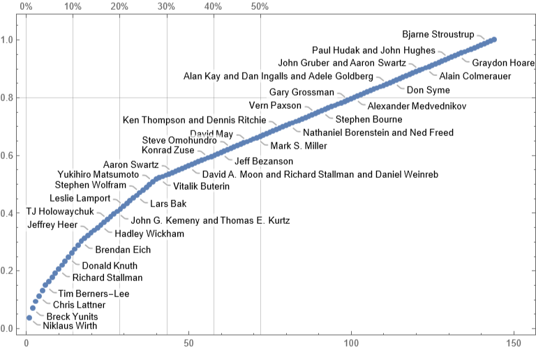
We can see that ≈25% of the creators correspond to ≈50% of the languages.
Popularity
Popularity
Obviously, programmers can and do use more than one programming language. Nevertheless, it is interesting to see the Pareto principle plot for the languages "mind share" based on the number of users estimates.
Remark: Again, the plot above is "wrong" -- programmers use more than one programming language.
Correlations
Correlations
In order to see meaningful correlation, pairwise plots we take logarithms of the large value columns:
Remark: Note that we "cheat" by adding 1 before taking the logarithms.
We obtain the tables of correlations plots using the newly introduced, experimental PairwiseListPlot. If we remove the rows with zeroes some of the correlations become more obvious. Here is the corresponding tab view of the two correlation tables:
Remark: Given the names of the data columns and the corresponding obvious interpretations we can say that the stronger correlations make sense.
Bubble chart 2D
Bubble chart 2D
In this section we make an informative 2D bubble chart with (tooltips).
First, note that not all triplets of "appeared","ageAtCreation", and "numberOfUsersEstimate" are unique:
Hence we make two datasets: (1) one for the core bubble chart, (2) the other for the labeling function:
Here is the bubble chart:
Remark: The programming language J is a clear outlier because of creators' ages.
Bubble chart 3D
Bubble chart 3D
In this section we a 3D bubble chart.
As in the previous section we define two datasets: for the core plot and for the tooltips:
Here is the corresponding labeling function:
Make a bubble 3D chart:
Make a 3D plot with custom callouts:
Here is the combined 3D chart:
Remark: In the 3D bubble chart plot "Mathematica" and "Wolfram Language" are easier to discern.
Second system effect traces
Second system effect traces
In this section we try -- and fail -- to demonstrate that the more programming languages a team of creators makes the less successful those languages are. (Maybe, because they are more cumbersome and suffer the Second system effect?)
Remark: This section is mostly made "for fun." It is not true that each sets of languages per creators team is made of comparable languages. For example, complementary languages can be in the same set. (See, HTTP, HTML, URL.) Some sets are just made of the same language but with different names. (See, Perl 6 and Raku, and Mathematica and Wolfram Language.) Also, older languages would have the First mover advantage.
Make creators to index association:
Make a bubble chart with relative popularity per creators team:
From the plot above we cannot decisively say that:
The most recent creation of a team of programming language creators is not team’s most popular creation.
That statement, though, does hold for a fair amount of cases.
Instead of conclusions
Instead of conclusions
Consider:
◼
Making an interactive interface for the variables, types of plots, etc.
◼
Placing callouts for the focus languages in bubble charts.
References
References
Here are reference links with explanations and links to dataset files:
◼
◼
"Just a plot"; provides a link to a CSV file with the data.
◼
Link(s) and discussion.
CITE THIS NOTEBOOK
CITE THIS NOTEBOOK
Computational exploration for the ages of programming language creators dataset
by Anton Antonov
Wolfram Community, STAFF PICKS, May 21, 2024
https://community.wolfram.com/groups/-/m/t/3180327
by Anton Antonov
Wolfram Community, STAFF PICKS, May 21, 2024
https://community.wolfram.com/groups/-/m/t/3180327