A family member has taken up some amateur woodworking. While I was on break from my university, I had the opportunity to try a set of puzzle cubes that he had created. Naturally, after spending some time engaged with the puzzles, my mind turned to the question of how they could be solved programmatically using my favorite all-purpose computational software. Coming to a solution in Mathematica was every bit as rewarding as working on the puzzles manually, and the result is far more generalizable.
Background
Background
Puzzle Description
Puzzle Description
A polycube puzzle consists of a set of pieces that are fitted together to form a solid cube. Each piece is called a polycube because it is formed from multiple smaller cubes, called unit cubes, that are connected to one another. For example, each of the colored shapes shown below is a puzzle piece made of unit cubes, and when they are joined in exactly the right way, all of the pieces will combine into a single large cube. Below is an example of a polycube puzzle made out of wood. Note that the individual unit cubes are not marked but still define the shape of each piece.
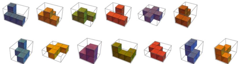
Polycube Puzzle Example
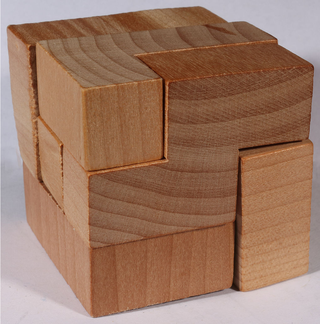
“Cube 3x3” by Wikimedia Commons user NottiP licensed under Creative Commons Attribution - Share Alike 3.0 Unported
Common polycube puzzles include the Soma cube, Bedlam cube, and Diabolical cube.
Representation as an Exact Cover Problem
Representation as an Exact Cover Problem
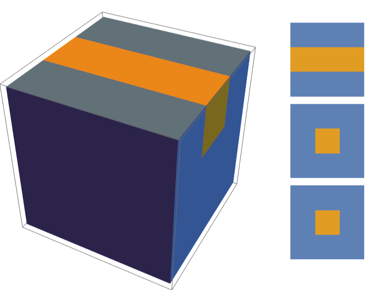
The exact cover problem is an NP-complete problem that refers to the task of finding subsets of a set such that the union of the subsets contains all elements of the set, but no two subsets share any common elements. Donald Knuth’s Dancing Links (DLX) algorithm is among the most effective algorithms for finding a solution to the exact cover problem. Despite the problem’s exponential time complexity in the worst case, DLX is often able to achieve much better scaling in practice. It is known that solving a polycube puzzle is equivalent to the exact cover problem. Indeed, Knuth’s original paper on DLX tested the algorithm’s efficiency on polyomino tiling, a 2D cousin of the puzzle. To solve a polycube puzzle using the exact cover problem, we must first know all of the pieces and the size of the final cube (the size of the cube could be derived from the sum of the piece sizes). Our goal is to create a binary occupancy matrix whose set cover can be found using DLX. We imagine that there is an empty space with the size and shape of the final cube. We then create one row of the occupancy matrix for each possible position where the first puzzle piece can be placed in the space. Each row consists of two sections. The first has length equal to the number of pieces in the puzzle and is a one-hot vector that serves to identify which piece is represented by this row. For all of the rows created for the first piece, the first position in this vector is a 1 and the remainder are 0s. The second section has length equal to the total number of unit cubes in the puzzle. For instance, it would be length 27 for a 3x3x3 cube and 64 for a 4x4x4 cube. Each position in the vector represents whether a specific unit cube position is filled (if 1) or unfilled (if 0) given the piece position represented by that row. We then repeat the procedure for the second and all later pieces. As a concrete example of this, we will use a very simple polycube puzzle with only two pieces. We can see that the solution to the puzzle should be as follows. The cube on the left shows the 3D view of the solution, and the three squares on the right show the cross sections of the top, middle, and bottom layers. To solve the puzzle by finding an exact cover, we must create the binary matrix described above.
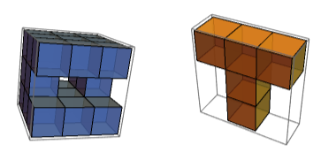
This matrix has 48 rows and 29 columns. The first two columns correspond to the two pieces while the remaining columns correspond to the 27 unit cubes in a 3x3x3 puzzle as described above. The rows beginning with “10” correspond to the 12 possible positions that the blue piece could occupy inside an empty 3x3x3 cube while the rows beginning with “01” correspond to the 36 positions that the orange piece could occupy.
We then compute an exact cover of this matrix, which is a list of rows of the matrix such that each column is filled by a 1 in exactly one row of the solution and by 0 in the others. The number of rows in the solution will be equal to the number of pieces in the puzzle and each represents the location of a piece.
We then compute an exact cover of this matrix, which is a list of rows of the matrix such that each column is filled by a 1 in exactly one row of the solution and by 0 in the others. The number of rows in the solution will be equal to the number of pieces in the puzzle and each represents the location of a piece.
{{1,0,1,1,1,1,0,1,1,1,1,1,1,1,1,0,1,1,1,1,1,1,1,0,0,0,1,1,1},{0,1,0,0,0,0,1,0,0,0,0,0,0,0,0,1,0,0,0,0,0,0,0,1,1,1,0,0,0}}
The code for this project is shown in the “Building a Polycube Puzzle Solver” section.
Notes on Occupancy Matrix Length
Notes on Occupancy Matrix Length
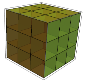
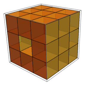
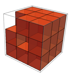
Pieces that are smaller and have less symmetry will have more placement possibilities within an empty cube than larger, symmetrical pieces. Thus, they will contribute more rows to the matrix. In a 3x3x3 puzzle, if an individual puzzle piece were also 3x3x3 there would only be one placement possibility, and thus the piece would only have one row in the matrix. (This is the most trivial case possible and corresponds to a puzzle with only one piece.) However, if a single unit cube is removed from the middle of one of the cube faces, the symmetry will be reduced and there will be six placement possibilities and six rows. This is because the face with the missing unit cube could be rotated so that it is on any of the six faces of the empty 3x3x3 cube space. If one cube is removed from the middle of a cube face and one is removed from a corner, the cube will have no symmetry and will add 24 rows to the matrix. The missing face cube could be on any of the six faces of the empty cube and this is multiplied by the four corners of that face where the missing corner could be located. If the piece size were reduced to 2x2x2 (with no missing unit cubes from the faces or corners), there would be 8 rows added. In each of the three dimensions, the 2x2x2 cube can be placed on either one side or the other of the 3x3x3 empty cube and thus we obtain possible placements.
3
2
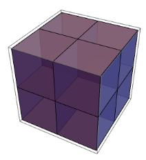
In general, a piece can be rotated in 24 different orientations, as shown in the image of the red cube with missing face and corner unit cubes above. However, symmetry can reduce this number as in the examples of the green and orange cubes. The number of orientations can then be multiplied by the number of possible locations of the piece within the larger, empty cube as shown in the example of the 2x2x2 purple cube. So an equation for the number of rows contributed by a piece is as follows.
24
γ
Here, s is the cube edge length (so s = 3 for a 3x3x3 cube), and a, b, and c are the edge lengths of the bounding box around the piece. For example, the piece shown here with its bounding box drawn around it has bounding box edge lengths of 1, 2, and 3.
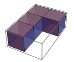
The variable γ represents the reduction in the unique number of piece orientations caused by symmetry. It must be true that γ is a factor of 24.
Building a Polycube Puzzle Solver
Building a Polycube Puzzle Solver
Implementation
Implementation
This section provides the code for a polycube puzzle solver in Mathematica with a graphical user interface.
The FindExactCover resource function will find an exact cover for the occupancy matrix once it has been created. It uses DLX for this by default.
Import the FindExactCover resource function:
In order to find all possible positions in which a piece can be placed, I first need to define how to rotate a piece in a specified direction.
I want to be able to standardize the puzzle pieces entered by the user so that they are adjacent to the origin, which is accomplished as follows.
The following function takes a piece that has been standardized to be adjacent to the origin and determines every possible placement of that piece within the empty cube with size equal to the completed puzzle size. This is needed in order to create the occupancy matrix as explained in the “Representation as an Exact Cover Problem” section.
The createOccupancyList function creates a single row of the occupancy matrix, not including the one-hot vector at the beginning of the row that specifies which piece the row belongs to.
The createOccupancyRows function creates the entire occupancy matrix with the exception of the one-hot vector at the beginning of each row.
The createOccupancyMatrix function creates the complete occupancy matrix including the one-hot vector.
I also define a function to convert the list representation of the pieces from the format received from the input to the GUI to a list of coordinates for use by the backend.
The puzzle can then be solved with input from the GUI.
A GUI is created to receive input and display output.
The solver can then be called directly in a notebook or deployed to Wolfram Cloud. If running the GUI in a notebook however, it is best to use the “DOWNLOAD-DESKTOP-NOTEBOOK.nb” attachment or copy the code into a fresh notebook rather than run it in the notebook downloaded from the “Get this Notebook” option at the bottom of this post. The notebook margins necessary for the community post do not leave much space for the GUI in the horizontal direction, so it is more pleasantly viewed in a notebook with more standard margins.
Usage
Usage
The GUI layout is shown here.
A cube size of 3, 4, or 5 can be selected on the top bar. (A puzzle smaller than size 3 would be trivial while those larger than size 5 are rare and have longer solve times. )
Puzzle pieces are created one at a time by selecting the grey squares and pressing the “Submit Piece” button.
The created puzzle piece appears below the “Submit Piece” button.
Once all pieces have been input, “Solve Puzzle” is pressed.
The output includes a large 3D representation of the exterior of the solved puzzle as well as cross-sections of the top, middle, and bottom layers of the solution.
The puzzle solved in this example was the Soma cube, a classic polycube puzzle.
Concluding Remarks
Concluding Remarks
This post explored a method of solving a class of puzzles whose pieces are composed of geometrical shapes known as polycubes. In this method, finding a puzzle solution is equivalent to finding an exact cover of an augmented occupancy matrix formed from the possible positions of the pieces within the puzzle. After an explanation of the principles behind this approach, code was provided to implement a puzzle-solving program in Mathematica along with an explanation of how to use the solver. It is hoped that this information will be of use to those interested in a programmatic solution to this variety of puzzle.
Acknowledgments
Acknowledgments
This project was greatly enhanced by the use of the FindExactCover function submitted to the Wolfram Function Repository by Brad Klee.
References
References
1
.Busche, M. (2011). “Solving Polyomino and Polycube Puzzles.” From Matt’s Maniacal Musings. https://www.mattbusche.org/blog/article/polycube/.
2
.Knuth, D. (2000). “Dancing Links.” Millenial Perspectives in Computer Science, 2000, 187--214. arXiv:cs/0011047.
CITE THIS NOTEBOOK
CITE THIS NOTEBOOK
Solving polycube puzzles by applying the exact cover problem
by Curran Flanders
Wolfram Community, STAFF PICKS, December 30, 2024
https://community.wolfram.com/groups/-/m/t/3346410
by Curran Flanders
Wolfram Community, STAFF PICKS, December 30, 2024
https://community.wolfram.com/groups/-/m/t/3346410