ABSTRACT (original article): Quasinormal modes and frequencies are the eigenvectors and eigenvalues of a nonHermitian differential operator. They hold crucial significance in the physics of black holes. The analysis of quasinormal modes of black holes in asymptotically Anti-de Sitter geometries plays also a key role in the study of strongly coupled quantum many-body systems via gauge/gravity duality. In contrast to normal Sturm-Liouville operators, the eigenvalues of non-Hermitian (and non-normal) operators generally exhibit instability under small perturbations. This research focuses on the stability analysis of quasinormal frequencies pertaining to asymptotically planar AdS black holes, employing pseudospectrum analysis. Specifically, we concentrate on the pseudospectra of scalar and transverse gauge fields, shedding light on their relevance within the framework of gauge/gravity duality. CITATION (original article): Areán, D., Fariña, D.G. & Landsteiner, K. Pseudospectra of holographic quasinormal modes. J. High Energ. Phys. 2023, 187 (2023). https://doi.org/10.1007/JHEP12(2023)187
1 Introduction
1 Introduction
Quasinormal modes (QNMs) are solutions of linear differential equations on an open domain. They can be thought of as the eigenmodes of linear differential operators satisfying outgoing boundary conditions demanded by the open nature of the domain. Due to these boundary conditions, the differential operator is non-Hermitian and the eigenvalues are complex.
In gravitational physics, QNMs appear when studying fluctuations about black hole backgrounds. As black hole horizon acts as a perfectly absorbing membrane, solving a wave equation in a black hole background leads naturally to outgoing boundary conditions. A particularly interesting case is that of QNMs in (asymptotically) Anti de-Sitter (AdS) spaces. Famously, gauge/gravity relates these spacetimes to certain strongly coupled quantum many-body systems [1-5]. Consequently, studying QNMs in AdS sheds light on the behaviour of excitations in the aforementioned quantum many-body systems. In particular, the characteristic frequencies of the QNMs, called quasinormal frequencies (QNFs), correspond to the spectrum of the excitations in the dual quantum-many body system.
A question that so far has not been investigated in the context of gauge/gravity duality is the stability of the quasinormal frequencies under small perturbations of the background geometry. In asymptotically flat spacetimes such studies have a long history [6, 7] and recently the issue has been taken up in [8–14] (see also [15] for horizonless compact objects). The key new development of these recent studies is the application of the method of pseudospectra [16].
The eigenvalues of Hermitian operators are stable in a technical sense. In fact, this stability is what makes perturbation theory successful in quantum physics. On the other hand, the eigenvalues of non-Hermitian and non-normal operators generically are unstable. This means they can be displaced large distances by even small perturbations of the original operator. In the case of quasinormal modes the instability appears as a consequence of the non-conservative nature of the system, associated with the outgoing boundary conditions. As the existence of an event horizon ensures these boundary conditions, is reasonable to expect that QNFs in AdS are also inherently unstable as occurs in asymptotically flat spacetimes. The motivation for investigating this question is twofold. Firstly, it would serve as increasing evidence of the independence of the instability on the asymptotic behaviour of the spacetime. And secondly, it would shed a completely new light on the behaviour of strongly coupled quantum many-body systems modelled by gauge/gravity duality. The instability of the quasinormal mode spectrum would indicate that also the excitation spectrum of the dual quantum field theories would be unstable under perturbations.
To probe the stability of the QNFs we follow the example of [8] and turn to pseudospectrum analysis [16]. Broadly speaking, pseudospectrum provides insight on how much perturbations of a given size can displace the spectrum of an operator. Accordingly, once the physically motivated notion of size is defined, pseudospectra serve as a powerful tool to discuss spectral stability or lack thereof.
In this notebook we analyze the stability of the QNMs associated with the transverse components of a U(1) gauge field in a Schwarzschild () background. This corresponds to one of the cases discussed in [17]. Here, we mainly focus on the computational aspects of the study, we refer the interested reader to the original work for a more detailed analysis of the physics. For simplicity, we choose to mainly focus on the zero momentum case. Nonetheless, in subsection 7.4 we compute the dependence of stability on momenta.
AdS
4+1
SAdS
4+1
Plots Parameters
Plots Parameters
2 Review of Pseudospectrum
2 Review of Pseudospectrum
In this section we give a very brief, heuristic introduction to the basic ideas and concepts of stability analysis through pseudospectra and condition numbers. For a more in-depth review, we refer the reader to [16].
In short, ε-pseudospectra and condition numbers allow us to address the following question: How much can the spectrum of a (closed linear) operator be displaced after a small perturbation of size ε ()? For a generic operator , this is a highly non-trivial question. However, if and its adjoint satisfy , i.e., if is normal, the spectrum is protected by the spectral theorem and thus the eigenvalues can be displaced at most a distance ε (meaning the spectrum is stable).
V
||V||=ε
L
L
†
L
[L,]=0
†
L
L
In physics, conservative systems are described using self-adjoint operators, which are trivially normal. Consequently, conservative systems have a stable spectrum. On the other hand, in non-conservative systems, the spectrum need not be stable since these systems are defined by non-self-adjoint operators that may be non-normal. Then, considering that any physical model is, by construction, a small deviation from nature, one must complement spectra in non-conservative systems with pseudospectra to properly grasp the predictivity of the model.
Now, let us focus on stability analysis for operators acting on a finite dimensional Hilbert space ℋ, i.e. matrices. We assume that the space is equipped with an inner product , which can be written as
<·,·>
<u,v>=Gv=Fv,
*
u
*
u
*
F
(
1
)where u* is the complex conjugate transpose of u, G is a matrix representing the inner product and F is the Cholesky decomposition of G.
We give two mathematically equivalent definitions ε-pseudospectra (M) of a matrix M
σ
ε
Def. 1 (Resolvent approach to pseudospectrum)
σ
ε
min
λ∈(A-z)
*
(A-z)
-1
FMF
(
2
)
Def. 2 (Perturbative approach to pseudospectrum)
Def. 2 (Perturbative approach to pseudospectrum)
σ
ε
(
3
)where denotes the spectrum and the operator norm V is defined by
σ(·)=(·)
σ
0
V=λ,B=
max
λ∈B
*
B
-1
FVF
(
4
)The first definition is the one that we will mainly use for computations throughout this notebook. However, the second one is the physically relevant one. It tells us the boundary of the ε-pseudospectra denotes the region where we might find an eigenvalue of M after a perturbation V of size . Interestingly, both definitions of pseudospectra are norm dependent. This was to be expected, in stability analysis one needs a “ruler” in order to determine what constitutes a small perturbation. Consequently, from a physical point of view we have to choose a well-motivated norm so that the physical notion of size matches the mathematical one induced by the norm.
||V||<ε
With regards to condition numbers of the spectrum of a matrix M, we have the following definition and theorem
{}
κ
i
Def. 3 (Condition numbers)
κ
i
v
i
2
u
i
2
<,
v
i
u
i
>
2
(
5
)where is the usual matrix -norm, the matrix -inner product and and satisfy the following eigenvalue equations
·
2
2
L
<·,·
>
2
2
L
v
i
u
i
-1
FMF
u
i
λ
i
u
i
*
()
-1
FMF
v
i
λ
i
v
i
(
6
)with the complex conjugate of .
Thm.1
Given a small perturbation of size ε, an eigenvalue of a matrix M can be displaced at most +O().
λ
i
λ
i
Thm.1
Given a small perturbation of size ε, an eigenvalue
λ
i
εκ
i
2
ε
Note that with this definition, condition numbers satisfy >=1, the equality only taking place when the eigenvalue is stable.
κ
i
Lastly, another important concept is the selective pseudospectrum. Both condition numbers and (full) pseudospectra probe the stability under generic perturbations. However, in many cases, it is more interesting to construct a selective pseudospectrum considering only a particular type of perturbations. In practice, this selective pseudospectrum is generated using definition 2, with the perturbations V being randomly-generated following some physically-motivated constraints.
3 Holographic Model
3 Holographic Model
In this section we define the fluctuations whose stability we are going to test. We consider fluctuations associated with the transverse components of a U(1) gauge fields in a background. The action is given by
M
SAdS
4+1
S[]=-∫x),
1
4
4+1
-g
(F
MN
MN
F
(
7
)where =- .
F
MN
∂
M
N
∂
N
M
We choose the regular coordinates (,x,ρ) presented in [17] for the background. The metric in these coordinates is given by
SAdS
4+1
2
ds
2
l
2
z
h
2
(1-ρ)
2
d
δ
ij
i
dx
j
dx
z
h
2
z
h
2
dρ
4
(1-ρ)
(
8
)where l is the AdS radius, = with the temperature of the black hole and and correspond to the event horizon and the AdS boundary, respectively. Remarkably, these coordinates allow us to fix outgoing (infalling towards the horizon) boundary conditions as regularity conditions on the event horizon while also producing an standard eigenvalue problem for the QNMs.
z
h
1
πT
T
ρ=0
ρ=1
It is important to note that the fields in (7) depend on the coordinates (,x,ρ). However, throughout the remainder of this notebook we will eliminate the x dependence by preforming a Fourier decomposition. Consequently, henceforth whenever explicit dependence is omitted we shall assume that the functions are functions of (,k,ρ).
It is also worth pointing out that, instead of working with dimensionful momentum k and quasinormal frequencies ω, we opt to introduce the dimensionless quantities and .
𝔮=k
z
h
𝔴=ω
z
h
As indicated in section 1 we will focus mostly on the case. Nonetheless, as we will also study the momentum dependence in subsection 7.4, we leave 𝔮 as a parameter to be fixed in each section.
𝔮=0
3.1 Equations of Motion and Energy Norm
3.1 Equations of Motion and Energy Norm
We first define the equations of motion for the QNMs and the physically motivated norm, the energy norm . For practical purposes, we find it convenient to define them in terms of the rescaled scalar doublet defined as
||·
||
E
at |
αt |
=
,
at |
αt |
-1
(1-ρ)
a |
α |
(
9
)where and “a” denotes a generic component of the transverse gauge field
α=a
z
h
∂
t
In[]:=
(*Equationsofmotionfortherescaledtransversegaugefield*)gfEOMs=𝔴at[ρ]-αt[ρ],𝔴αt[ρ]-+4++3(-2+ρ)ρ(2+(-2+ρ)ρ)at[ρ]+(-1+ρ)((4+5(-2+ρ)ρ(2+(-2+ρ)ρ))[ρ]+(-2+ρ)(-1+ρ)ρ(2+(-2+ρ)ρ)[ρ])((2+(-2+ρ)ρ(2+(-2+ρ)ρ)));(*Integrandoftheenergynormfortherescaledtransversegaugefield*)gfEnorm=-((-1+ρ)(2-4ρ+6-4+)αt[ρ]αtb[ρ])+(-2+ρ)ρ(2-2ρ+)[ρ](atb[ρ]+(-1+ρ)[ρ])+at[ρ]-+ρ(-4+6ρ-4+)atb[ρ]+ρ(4-10ρ+10-5+)[ρ];gfu={at[ρ],αt[ρ]};gfbu={atb[ρ],αtb[ρ]};
(5αt[ρ]+2(-1+ρ)[ρ])
3
(-1+ρ)
′
αt
2+(-2+ρ)ρ(2+(-2+ρ)ρ)
2
𝔮
2
(-1+ρ)
′
at
′′
at
2
(-1+ρ)
2
ρ
3
ρ
4
ρ
2
ρ
′
at
′
atb
1
-1+ρ
2
𝔮
2
(-1+ρ)
2
ρ
3
ρ
2
ρ
3
ρ
4
ρ
′
atb
Remarkably, in terms of the rescaled doublet, the equation of motion for the QNMs can be written as an eigenvalue problem and the desired asymptotic behaviour
a[ρ->1]∝,n>1
n
(𝜌−1)
(
10
)can be imposed as a Dirichlet boundary condition on the AdS boundary. Furthermore, the energy norm is positive definite and finite for all regular functions with the asymptotic behaviour (10).
4 Discretization
4 Discretization
We approach the stability analysis numerically; discretizing the radial coordinate ρ in a Chebyshev grid. Consequently, in this section we construct the function PseudoSpectrumSetup, which generates the discretized version of the equations of motion and the norm. As inputs, PseudospectrumSetup takes: equations of motion: eoms norm: norm Rescaled fields: u Rescaled complex conjugated fields: bu Grid size - 1: n Precision: precision and the flowchart is given by
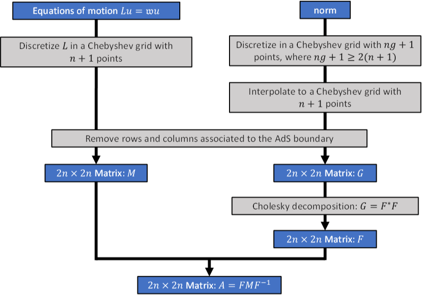
Note that when constructing the G matrix, which corresponds to the discretized version of the norm, we have to first construct it in a larger grid and then interpolate back to our grid with points. This ensures that the norm is exact for polynomials of degree . A detailed discussion of this subtlety can be found in appendix B of [17].
n+1
n
SetDirectory[NotebookDirectory[]];PseudoSpectrumSetup[eoms_,norm_,u_,bu_,n_,precision_]:=Module{Nfields,Mterm,Mij,Gterm,GtermD,Gngij,Gij,G2ij},Nfields=Length[eoms];If[Nfields!=Length[u],Throw["Error: Number of equations does not match the number of fields"]];LaunchKernels[];(*-----------------------QNMsystemdefinition-----------------------*)(*griddefinition*)ρgrid=SetPrecision(1-Cos[πRange[0,n,1]/n]),2*precision;(*Chebyshevderivativematrices*)DN=NDSolve`FiniteDifferenceDerivative[1,ρgrid,"DifferenceOrder""Pseudospectral",PeriodicInterpolationFalse]["DifferentiationMatrix"];DN2=NDSolve`FiniteDifferenceDerivative[2,ρgrid,"DifferenceOrder""Pseudospectral",PeriodicInterpolationFalse]["DifferentiationMatrix"];(*-----------------ConstructionofM-----------------*)M=Array[Mij,{Nfields,Nfields}];SetSharedFunction[Mij];(*asthepointn+1correspondstotheAdSboundary,weremoveittoimposeDirichletboundaryconditions*)ParallelTableMterm[i]=-Coefficienteoms[[i]],𝔴,0//FullSimplify;Mij[i,j]=SetPrecision[DiagonalMatrix[(Coefficient[Mterm[i],u[[j]]]/.ρ->ρgrid[[1;;n]])+0*ρgrid[[1;;n]]]+DiagonalMatrix[(Coefficient[Mterm[i],D[u[[j]],{ρ,1}]]/.ρ->ρgrid[[1;;n]])+0*ρgrid[[1;;n]]].DN[[1;;n,1;;n]]+DiagonalMatrix[(Coefficient[Mterm[i],D[u[[j]],{ρ,2}]]/.ρ->ρgrid[[1;;n]])+0*ρgrid[[1;;n]]].DN2[[1;;n,1;;n]],precision];,{i,1,Nfields},{j,1,Nfields};M=Flatten[M,{{1,3},{2,4}}];(*-----------------------Energynorm-----------------------*)(*extendedgriddefinition*)ng=2*n+10;ρgridng=SetPrecision(1-Cos[πRange[0,ng,1]/ng]),2*precision;(*Chebyshevderivativematrix*)DNg=NDSolve`FiniteDifferenceDerivative[1,ρgridng,"DifferenceOrder""Pseudospectral",PeriodicInterpolationFalse]["DifferentiationMatrix"];(*Weightmatrix*)GWg=SetPrecisionDiagonalMatrixParallelTableSum-,{k,0,ng,2},{i,0,ng},precision;(*Interpolarionmatrix*)InterpFROMnTOng=SetPrecisionParallelTable*SumChebyshevT[k,2ρgrid[[j+1]]-1],{k,0,n},{i,0,ng},{j,0,n},precision;(*ConstructionofGwithDirichletboundaryconditions*)G=Array[Gij,{Nfields,Nfields}];SetSharedFunction[Gij];ParallelTable[Gterm[i]=Coefficient[norm,bu[[i]]]//FullSimplify;GtermD[i]=Coefficient[norm,D[bu[[i]],{ρ,1}]]//FullSimplify;Gngij[i,j]=DiagonalMatrix[Join[((Coefficient[Gterm[i],u[[j]]]/.ρ->ρgridng[[1;;ng]])+0*ρgridng[[1;;ng]]),{0}]].GWg+DiagonalMatrix[Join[((Coefficient[Gterm[i],D[u[[j]],{ρ,1}]]/.ρ->ρgridng[[1;;ng]])+0*ρgridng[[1;;ng]]),{0}]].GWg.DNg+Transpose[DNg].DiagonalMatrix[Join[((Coefficient[GtermD[i],u[[j]]]/.ρ->ρgridng[[1;;ng]])+0*ρgridng[[1;;ng]]),{0}]].GWg+Transpose[DNg].DiagonalMatrix[((Coefficient[GtermD[i],D[u[[j]],{ρ,1}]]/.ρ->ρgridng)+0*ρgridng)].GWg.DNg;Gij[i,j]=(Transpose[InterpFROMnTOng].Gngij[i,j].InterpFROMnTOng)[[1;;n,1;;n]];,{i,1,Nfields},{j,1,Nfields}];G=Flatten[G,{{1,3},{2,4}}];(*ConstructionofF*)F=CholeskyDecomposition[G];(*Constructionof*)invF=Inverse[F];(*-----------------------ConstructionofA-----------------------*)A=F.M.invF;CloseKernels[];
1
2
1
2
2/ng
1+KroneckerDelta[i,0]+KroneckerDelta[i,ng]
1
(-1+)
2
k
ChebyshevT[k,2ρgridng[[i+1]]-1]
1+KroneckerDelta[k,0]+KroneckerDelta[k,ng]
1
(1+KroneckerDelta[j,0]+KroneckerDelta[j,n])*n
2ChebyshevT[k,2ρgridng[[i+1]]-1]
(1+KroneckerDelta[k,0]+KroneckerDelta[k,n])
-1
F
A few comments regarding the code are in order. First, note that the grid and the Chebyshev derivative matrices are constructed with twice the specified precision. This reduces the effect of error propagation and ensures that the final results are indeed of the specified precision. Second, in the construction of the Gij blocks of the G matrix, we already impose Dirichlet boundary conditions by writing a zero in all terms that would appear multiplying the fields. This prevents the appearance of spurious “indeterminate entries” in the matrix, which would be associated to modes without the desired asymptotic behaviour.
5 Convergence Test
5 Convergence Test
Physically, the discretization and numerical round-offs can be understood as perturbations to the original problem and, as we want to analyze the stability of the latter, we need to be especially careful and avoid undesired effects associated with them. As we are mainly interested in the stability of the three or four lowest-lying QNFs, in this section we test the validity of our numerics by computing those QNFs in our setup and comparing them to the ones obtained using 10×MachinePrecision in a grid of 400 points.
Concretely, we fix the precision to be 5×MachinePrecision and, for different grid sizes, we compute the error defined as
6 Optimizing the Discretization
6 Optimizing the Discretization
With this in mind, in order to optimize the algorithm, it is convenient to construct and save a few objects that are model independent. These objects are the grids, the weight matrix, the interpolation matrix and Chebyshev derivative matrices.
7 Results for the Transverse Gauge Field
7 Results for the Transverse Gauge Field
We commence in subsection 7.1 by computing the full pseudospectrum and condition numbers as indicated in section 2. These results let us probe the overall stability of the system under arbitrary perturbations. However, from a physical standpoint, we are particularly interested in also analyzing the stability of the system under local potential perturbations appearing in the action as a term:
Remarkably, although in general this term would break the U(1) gauge symmetry, for the transverse sector it does not. This is associated with the fact that the transverse components of the gauge field are gauge invariant.
In order to obtain the stability under perturbations of the form (12), we compute the selective pseudospectrum of local potential perturbations in subsection 7.2. To further explore the effect of local perturbations, in subsection 7.3 we consider the following deterministic potentials
and study their effect on the QNFs. Note that we have introduced normalization constants to fix the magnitude of the perturbations. We present a plot the potentials bellow.
In subsection 7.4 we address the momentum dependence by computing the the condition numbers for the 3 lowest QNFs as a function of momentum.
Lastly in subsection 7.5 we collect the results and very briefly discuss their implications.
7.1 Full Pseudospectrum and Condition numbers
7.1 Full Pseudospectrum and Condition numbers
The full pseudospectrum, is represented by a heat map of the boundaries of the different ε-pseudospectra. Thus, an isothermal line denotes the boundary of the region where we might find the eigenvalues after a perturbation of the indicated size (or smaller). From a computational perspective, this is obtained by computing
in each point 𝔴 of the complex plane. This way, all points with the same ϵ correspond to the same ϵ-pseudospectrum boundary.
We choose to compute the pseudospectrum only in the physically relevant region of the complex plane containing the 4 lowest lying (pairs of) QNFs. Moreover, as the lowest lying QNF is particularly interesting due to its role on the low energy dynamics of the dual quantum many-body system, we also compute a closeup of the pseudospectrum around that QNF.
and then we compute the condition number as
To optimize the code, we find it convenient to employ Arnoldi iteration in the computation of eigenvalues and eigenvectors. Furthermore, in the pseudospectrum, we exploit it’s symmetry under reflections along the imaginary axis to compute it only in the in the Im(𝔴)>0 plane and then perform a reflection to obtain the Im(𝔴)<0 plane.
Construction of Full Pseudospectrum
Construction of Full Pseudospectrum
7.2 Selective Pseudospectrum
7.2 Selective Pseudospectrum
The form of the perturbation matrices comes trivially from rewriting the equations of motion introduced in subsection 3.1 in the presence of the potential term (12) with V[ρ]=(1-ρ)U[ρ]. Concretely, the perturbed equations of motion take the form
which allows us to conclude that the perturbation matrix is given by:
For consistency, we choose U[ρ] to be randomly generated and leave all the prefactors appearing in (18).
7.3 Deterministic Potentials
7.3 Deterministic Potentials
In this case, we also find the condition numbers for the perturbed system to be physically interesting. They tell us about the stability of the perturbed setup under generic arbitrary perturbations. In particular, in subsection 7.5 we will compare these condition numbers against the ones for the unperturbed system.
7.4 Momentum Dependence
7.4 Momentum Dependence
In order to analyze the dependence of the stability on momentum, we proceed to study the condition numbers as a function of 𝔮.
Computationally, this is achieved trough a loop in 𝔮, where in each iteration the condition numbers are computed as indicated in subsection 7.2 and then stored in an array. For simplicity, we limit ourselves to computing the condition numbers only for the 3 lowest-lying (pairs of) QNFs.
7.5 Final Results and Physical Interpretation
7.5 Final Results and Physical Interpretation
In this subsection we collect all the data computed throughout this section and generate plots which whose physics we briefly discuss.
First we plot condition numbers and pseudospectrum for the 4 lowest-lying QNFs.
Let us discuss the stability under arbitrary perturbations. We observe that the full ε-pseudospectra are characterized by large open regions containing multiple QNFs for small values of ε. This indicates that the QNFs are unstable under generic perturbations, a fact further confirmed by the condition numbers, which are all greater than 1. Moreover, we observe that instability increases the further away the QNFs are from the real axis. This can be seen from the condition numbers, which increase as we go to higher QNFs, and the full pseudospectrum, where for the higher QNFs we observe larger ε-pseudospectrum boundaries for smaller values of ε.
Regarding the stability under local potential perturbations. Remarkably, the selective pseudospectra also signal instability of the QNFs under these perturbations. However, the QNFs are less unstable under local potential perturbations. This can be seen from the scale difference, generic perturbations can have effects much larger than local potential perturbations of the same size. Physically, this indicates that the instability of the QNFs is mostly associated with non-local interactions.
Now we turn our attention to the stability of the first QNF, which has the smallest imaginary part and thus dominates the long time behaviour of the system. We proceed by plotting a closeup of the full and selective pseudospectra
Following this analysis of the deterministic potentials, we now present the spectrum and the condition numbers for the first 4 QNMs in the perturbed system with deterministic potentials (13).
Lastly we discuss the evolution of stability with momentum. To do so, we present a plot of the condition numbers as a function of 𝔮 for the first three QNFs.
Figure 5. Momentum dependence of the condition numbers of the first three transverse gauge field QNFs.
Remarkably, we find that as the momentum 𝔮 increases the condition numbers, and consequently the instability, decreases. This can be understood assuming a relation between distance to the real axis and instability. As we see in figure 6, for each QNF the imaginary part increases as 𝔮 increases and thus they become more stable.
Figure 6. Momentum dependence of the imaginary part of the first three transverse gauge field QNFs.
8 Conclusions
8 Conclusions
Lastly, it is important to reiterate that the main objective of this notebook was to illustrate the computational aspects of [17]. Consequently, while there is a brief discussion of the physics in subsection 7.5, many aspects have been omitted. In particular, we have not discussed the physical motivation behind the energy norm and the regular coordinates. For an in-depth discussion of these topics, we refer the reader to the original work.
References
References
[1] J. M. Maldacena, The Large N limit of superconformal field theories and supergravity, Adv. Theor. Math. Phys. 2 (1998) 231–252 [hep-th/9711200].
[2] O. Aharony, S. S. Gubser, J. M. Maldacena, H. Ooguri and Y. Oz, Large N field theories, string theory and gravity, Phys. Rept. 323 (2000) 183–386 [hep-th/9905111].
[3] M. Ammon and J. Erdmenger, Gauge/gravity duality: Foundations and applications. Cambridge University Press, Cambridge, 4, 2015.
[4] J. Zaanen, Y. Liu, Y. Sun and K. Schalm, Holographic Duality in Condensed Matter Physics. Cambridge University Press, 2015.
[5] S. A. Hartnoll, A. Lucas and S. Sachdev, Holographic Quantum Matter. MIT Press, 2018.
[6] H.-P. Nollert, About the significance of quasinormal modes of black holes, Phys. Rev. D 53 (1996) 4397–4402 [gr-qc/9602032].
[7] H.-P. Nollert and R. H. Price, Quantifying excitations of quasinormal mode systems, J. Math. Phys. 40 (1999) 980–1010 [gr-qc/9810074].
[8] J. L. Jaramillo, R. P. Macedo and L. Al Sheikh, Pseudospectrum and Black Hole Quasinormal Mode Instability, Phys. Rev. X 11 (2021), no. 3 031003 [2004.06434].
[9] K. Destounis, R. P. Macedo, E. Berti, V. Cardoso and J. L. Jaramillo, Pseudospectrum of Reissner-Nordström black holes: Quasinormal mode instability and universality, Phys. Rev. D 104 (2021), no. 8 084091 [2107.09673].
[10] S. Sarkar, M. Rahman and S. Chakraborty, Perturbing the perturbed: Stability of quasi-normal modes in presence of a positive cosmological constant, 2304.06829.
[11] M. H.-Y. Cheung, K. Destounis, R. P. Macedo, E. Berti and V. Cardoso, Destabilizing the Fundamental Mode of Black Holes: The Elephant and the Flea, Phys. Rev. Lett. 128 (2022), no. 11 111103 [2111.05415].
[12] E. Berti, V. Cardoso, M. H.-Y. Cheung, F. Di Filippo, F. Duque, P. Martens and S. Mukohyama, Stability of the fundamental quasinormal mode in time-domain observations against small perturbations, Phys. Rev. D 106 (2022), no. 8 084011 [2205.08547].
[13] R. A. Konoplya and A. Zhidenko, First few overtones probe the event horizon geometry, 2209.00679.
[14] A. Courty, K. Destounis and P. Pani, Quasinormal mode (in)stability and strong cosmic censorship, 2307.11155.
[15] V. Boyanov, K. Destounis, R. Panosso Macedo, V. Cardoso and J. L. Jaramillo, Pseudospectrum of horizonless compact objects: A bootstrap instability mechanism, Phys. Rev. D 107 (2023), no. 6 064012 [2209.12950].
[16] L. N. Trefethen and M. Embree, Spectra and Pseudospectra. Princeton University Press, Princeton, 2005.
[17] D. Arean, D. Garcia-Fariña and K. Landsteiner, Pseudospectra of Holographic Quasinormal Modes, 2307.08751
CITE THIS NOTEBOOK
CITE THIS NOTEBOOK
Pseudospectra of Holographic Quasinormal Modes
by David García Fariña
Wolfram Community, STAFF PICKS, August 30, 2023
https://community.wolfram.com/groups/-/m/t/3002089
by David García Fariña
Wolfram Community, STAFF PICKS, August 30, 2023
https://community.wolfram.com/groups/-/m/t/3002089