CITE THIS NOTEBOOK: Transmon qubit readout fidelity at threshold for quantum error correction by Liangyu Chen. Wolfram Community April 4 2023.
ORIGINAL ARTICLE: Chen, L., Li, HX., Lu, Y. et al. Transmon qubit readout fidelity at the threshold for quantum error correction without a quantum-limited amplifier. npj Quantum Information 9, 26 (2023). https://doi.org/10.1038/s41534-023-00689-6.
ORIGINAL ARTICLE: Chen, L., Li, HX., Lu, Y. et al. Transmon qubit readout fidelity at the threshold for quantum error correction without a quantum-limited amplifier. npj Quantum Information 9, 26 (2023). https://doi.org/10.1038/s41534-023-00689-6.
Article Abstract: High-fidelity and rapid readout of a qubit state is key to quantum computing and communication, and it is a prerequisite for quantum error correction. We present a readout scheme for superconducting qubits that combines two microwave techniques: applying a shelving technique to the qubit that reduces the contribution of decay error during readout, and a two-tone excitation of the readout resonator to distinguish among qubit populations in higher energy levels. Using a machine-learning algorithm to post-process the two-tone measurement results further improves the qubit-state assignment fidelity. We perform single-shot frequency-multiplexed qubit readout, with a 140ns readout time, and demonstrate 99.5% assignment fidelity for two-state readout and 96.9% for three-state readout–without using a quantum-limited amplifier.
Introduction
Introduction
State-of-the-art superconducting circuits have shown great potential as the leading platform of quantum computing, as demonstrated by the recent progress from Google including scalable quantum error correction as well as the quantum supremacy in 2019. In this work, we will focus on high-fidelity and rapid readout of a qubit state, which is key to quantum computing and communication, and it is a prerequisite for quantum error correction. We present a readout scheme for superconducting qubits that combines two microwave techniques: applying a shelving technique to the qubit that reduces the contribution of decay error during readout, and a two-tone excitation of the readout resonator to distinguish among qubit populations in higher energy levels. Using a machine-learning algorithm to post-process the two-tone measurement results further improves the qubit-state assignment fidelity. We perform single-shot frequency-multiplexed qubit readout, with a 140ns readout time, and demonstrate 99.5% assignment fidelity for two-state readout and 96.9% for three-state readout–without using a quantum-limited amplifier.
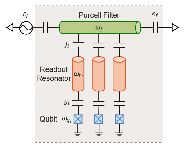
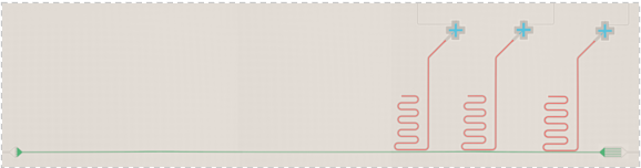
Here are the design scheme and optical micrograph of the physical device. Our device consists of three fixed-frequency transmon qubits each couple to a respective readout resonator. All three resonators are then coupled to the common Purcell filter embedded in the feedline. The measurements are done without a quantum-limited parametric amplifier in the readout chain.
Here are the design scheme and optical micrograph of the physical device. Our device consists of three fixed-frequency transmon qubits each couple to a respective readout resonator. All three resonators are then coupled to the common Purcell filter embedded in the feedline. The measurements are done without a quantum-limited parametric amplifier in the readout chain.
design=Image[Import[imgPath<>"Picture2.pdf"]〚1〛,Magnification->0.3]
device=Image[Import[imgPath<>"Picture1.png"],Magnification->1]
Initialization
Initialization
myred=ColorData[97][4];myblue=ColorData[97][1];myorange=ColorData[97][2];mygreen=ColorData[97][3];fontsize=14;font="CMU Sans Serif";SetOptions[EvaluationNotebook[],StyleDefinitionsCell[StyleData["GraphicsLabel"],Black,fontsize,FontFamilyfont]];gitPath="https://raw.githubusercontent.com/muxueqianxun/SuperconductingQubitReadout/main/";dataPath=gitPath<>"ReadoutData/";imgPath=gitPath<>"img/";
Readout Response
Readout Response
Import VNA Data
Import VNA Data
In[]:=
dataPathCalib=dataPath<>"Calibration/";dataVNAName=dataPathCalib<>"VNAZoom1.hdf5";
In[]:=
dataVNA=Import[dataVNAName,"/Traces/VNA - S21"];VNASignalWide=AbsArg[(dataVNA〚1〛)〚-2〛+I*(dataVNA〚2〛)〚-2〛];dataVNAStart=Import[dataVNAName,"/Step config/VNA - Start frequency/Step items"]〚1〛["single"];dataVNAStop=Import[dataVNAName,"/Step config/VNA - Stop frequency/Step items"]〚1〛["single"];dataVNAStep=Import[dataVNAName,"/Step config/VNA - # of points/Step items"]〚1〛["single"];
In[]:=
freqSweep=Range[dataVNAStart,dataVNAStop,Abs[(dataVNAStop-dataVNAStart)]/(dataVNAStep-1)];dataPhase=VNASignalWide〚All,2〛;cut=Round[0.59*dataVNAStep];cut1=Round[0.2*dataVNAStep];dataVNA=freqSweep,20*Log10[VNASignalWide〚All,1〛];dataVNASmooth=MovingAverage[dataVNA,2000];
9
10
Purcell Filter
Purcell Filter
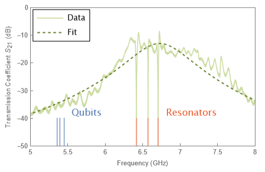
To characterize our device, we first look at the S21 parameter as a function of frequency. Our qubits sits at 5.3 GHz and the respective resonators are at 6.5 GHz, the peak of the profile here is the center of the Purcell filter, which is around 6.4 GHz.
In[]:=
bSol=Solve[0-I*Δ*b-κf/2*b-I*ϵf(*-γb*b*),b]〚1〛;
In[]:=
modelf=Simplify20*Log10*b*/.bSol1/.{Δf-ωp},{ϵf∈Reals,f∈Reals,κf∈Reals,γb∈Reals,ωp∈Reals};
2
κf
4
b
In[]:=
cut=Round[0.75*dataVNAStep];cut1=Round[0.35*dataVNAStep];cut2=Round[0.56*dataVNAStep];cut3=Round[0.78*dataVNAStep];dataVNASmoothCut=dataVNASmooth〚cut1;;cut2〛;dataVNASmoothCut1=dataVNASmooth〚cut;;-1〛;dataVNASmoothCutL=dataVNASmooth〚cut1;;cut3〛;dataVNASmoothCut2=Join[dataVNASmoothCut,dataVNASmoothCut1];
In[]:=
resultf=NonlinearModelFit[dataVNASmoothCutL,modelf,{{ωp,6.5},{κf,0.4}(*,{γb,0}*),{ϵf,1}},f,MaxIterations1000];
In[]:=
imsize=395;qbList={5.357555,5.35755,5.39357,5.39357,5.45141,5.45141};roList={6.45311`,6.45311`,6.60611`,6.60611`,6.74131`,6.74131`}-0.036;line={-40,-60,-40,-60,-40,-60};qubitline=Partition[{qbList,line},2];roline=Partition[{roList,line},2];fitplotf=Legended[Show[ListPlot[{dataVNA},JoinedTrue,PlotRange{{5,8},{0,-50}},GridLinesAutomatic,FrameTrue,ImageSizeimsize,FrameTicks{{Range[-50,0,10],None},{Range[5,8,0.5]/.{5.5,6.6,7.7,8.8},None}},PlotStyle{{Lighter[Lighter[mygreen]],Thickness[0.004]}},FrameLabel{"Frequency (GHz)","Transmission Coefficient (dB)"},Epilog{{Text[Style["Qubits",fontsize,myblue,FontFamilyfont],{5.75,-38}]},{Text[Style["Resonators",fontsize,myred,FontFamilyfont],{7.15,-38}]}},ImageMargins0],ListPlot[qubitline,JoinedTrue,PlotStyle{Lighter[myblue]}],ListPlot[roline,JoinedTrue,PlotStyle{Lighter[myred]}],Plot[resultf[f],{f,dataVNA〚1,1〛,dataVNA〚-1,1〛},PlotStyle{Darker[mygreen],Dashed}]],Placed[Framed[LineLegend[{Lighter[Lighter[mygreen]],{Darker[mygreen],Dashed}},{"Data","Fit"},LabelStyle{FontFamilyfont}],BackgroundWhite,FrameMargins0.1],{Left,Top}]]
S
21
Resonator 2 Zoom-in
Resonator 2 Zoom-in
Import Data
Import Data
In[]:=
dataRQA=Import[dataPathCalib<>"Q1Q2Q3SSRO123pulseROSweep_3.hdf5","/Data/Data"];r1sweep=dataRQA〚All,3,1〛*;r2sweep=dataRQA〚All,4,1〛*;r3sweep=dataRQA〚All,5,1〛*;
-9
10
-9
10
-9
10
In[]:=
r1g=#〚1〛+I*#〚2〛&/@Partition[Flatten[dataRQA〚All,-6;;-5〛]〚1;;;;4〛,2];r1e=#〚1〛+I*#〚2〛&/@Partition[Flatten[dataRQA〚All,-6;;-5〛]〚2;;;;4〛,2];r1f=#〚1〛+I*#〚2〛&/@Partition[Flatten[dataRQA〚All,-6;;-5〛]〚3;;;;4〛,2];r1h=#〚1〛+I*#〚2〛&/@Partition[Flatten[dataRQA〚All,-6;;-5〛]〚4;;;;4〛,2];r2g=#〚1〛+I*#〚2〛&/@Partition[Flatten[dataRQA〚All,-4;;-3〛]〚1;;;;4〛,2];r2e=#〚1〛+I*#〚2〛&/@Partition[Flatten[dataRQA〚All,-4;;-3〛]〚2;;;;4〛,2];r2f=#〚1〛+I*#〚2〛&/@Partition[Flatten[dataRQA〚All,-4;;-3〛]〚3;;;;4〛,2];r2f=#〚1〛+I*#〚2〛&/@Partition[Flatten[dataRQA〚All,-4;;-3〛]〚3;;;;4〛,2];r2h=#〚1〛+I*#〚2〛&/@Partition[Flatten[dataRQA〚All,-4;;-3〛]〚4;;;;4〛,2];r3g=#〚1〛+I*#〚2〛&/@Partition[Flatten[dataRQA〚All,-2;;-1〛]〚1;;;;4〛,2];r3e=#〚1〛+I*#〚2〛&/@Partition[Flatten[dataRQA〚All,-2;;-1〛]〚2;;;;4〛,2];r3f=#〚1〛+I*#〚2〛&/@Partition[Flatten[dataRQA〚All,-2;;-1〛]〚3;;;;4〛,2];r3h=#〚1〛+I*#〚2〛&/@Partition[Flatten[dataRQA〚All,-2;;-1〛]〚4;;;;4〛,2];
In[]:=
r1gs={r1sweep,Abs[r1g]};r1es={r1sweep,Abs[r1e]};r1fs={r1sweep,Abs[r1f]};r1hs={r1sweep,Abs[r1h]};r2gs={r2sweep,Abs[r2g]};r2es={r2sweep,Abs[r2e]};r2fs={r2sweep,Abs[r2f]};r2hs={r2sweep,Abs[r2h]};r3gs={r3sweep,Abs[r3g]};r3es={r3sweep,Abs[r3e]};r3fs={r3sweep,Abs[r3f]};r3hs={r3sweep,Abs[r3h]};
In[]:=
r1gs〚All,2〛=20Log10[r1gs〚All,2〛];r1es〚All,2〛=20Log10[r1es〚All,2〛];r1fs〚All,2〛=20Log10[r1fs〚All,2〛];r1hs〚All,2〛=20Log10[r1hs〚All,2〛];r2gs〚All,2〛=20Log10[r2gs〚All,2〛];r2es〚All,2〛=20Log10[r2es〚All,2〛];r2fs〚All,2〛=20Log10[r2fs〚All,2〛];r2hs〚All,2〛=20Log10[r2hs〚All,2〛];r3gs〚All,2〛=20Log10[r3gs〚All,2〛];r3es〚All,2〛=20Log10[r3es〚All,2〛];r3fs〚All,2〛=20Log10[r3fs〚All,2〛];r3hs〚All,2〛=20Log10[r3hs〚All,2〛];
Readout Resonator Model
Readout Resonator Model
We then look at each resonator more closely and here is the state-dependent resonator response for qubit at 0,1,2 and 3 state. This measurement will be useful in choosing the optimal readout frequency in the later experiments that needs to readout out the higher energy state accurately.
Primary Tone IQ Plot
Primary Tone IQ Plot
Secondary Tone IQ Plot
Secondary Tone IQ Plot
Readout Resonator Model
Readout Resonator Model
Single-shot Readout IQ Data
Single-shot Readout IQ Data
Here are the measured results of the two readout tone respectively, plotted on a 2D IQ-plane.
Import IQ Data
Import IQ Data
Sample Training Data
Sample Training Data
Plot IQ Values
Plot IQ Values
Primary Tone
Primary Tone
Secondary Tone
Secondary Tone
Baseline Single-tone Assignment Fidelity
Baseline Single-tone Assignment Fidelity
We could calculate the baseline assignment fidelity by using the simple pointer state method, which assign the initial qubit state to each shot by the closest averaged center. We find an assignment fidelity of which is 94.3% in this particular measurement.
Pointer-state Classification
Pointer-state Classification
Re-construct and Plot Assignment Matrix
Re-construct and Plot Assignment Matrix
Neural Network
Neural Network
To analyze the two-tone results is to utilize a machine learning algorithm provided by Wolfram Mathematica.We combine the I and Q data from each tone into a 4-element vector and feed into a forward neural network,which contains 2 hidden layers.Then it could output the probability for the qubit to initially be at 0〉 , 1〉 or 2〉 state.The initial training of around a few minutes and the classification is also relatively fast. The reason why we favored the neural network over other algorithms such as support-vector machine(SVM) or non-linear support-vector machine(NSVM) is it’s scalability and better performance when discriminating more than two qubit states.
Train Neural Network
Train Neural Network
State Discrimination
State Discrimination
Here are the measured results of the two readout tone,and we combine them to reproduce the three-state assignment matrix.Average of the trace give us a three-state single-shot readout assignment fidelity of 97.0% with the two-tone readout pulse,achieving a significant improvement over the single-tone case,which is originally 94.3%. One special feature of this scheme is that the 2-state is less likely to be misidentified as 1-state than 0-state.Since 2 state is transfer to 1 state as a result of the additional pulses,it’s more easily to decay to 0 than be excited up to 2.
Preselection
Preselection
Classification
Classification
Optimize Confidence Thresholds
Optimize Confidence Thresholds
Re-construct Assignment Matrix
Re-construct Assignment Matrix
Plot Decision Boundary
Plot Decision Boundary
Primary Tone
Primary Tone
Secondary Tone
Secondary Tone
Conclusion
Conclusion
To sum it up, with a device designed with a common Purcell filter, we have achieved a boost in assignment fidelity of two-state and three-state readout by exploiting the higher energy levels and using the two-tone readout pulse, all without using a quantum-limited parametric amplifier. The technique is robust and straightforward to implement in current state-of-the-art superconducting devices.
We will continue to investigate the remaining error that limits our readout fidelity, which includes the errors in state preparation pulses, excitation from measurement-induced mixing and readout crosstalk and dephasing during multiplexed readout. Further improvements include using neural network to aid the optimization of the readout pulses, integrate unconditional reset protocol and utilize parametric amplifiers to further boost SNR.
We will continue to investigate the remaining error that limits our readout fidelity, which includes the errors in state preparation pulses, excitation from measurement-induced mixing and readout crosstalk and dephasing during multiplexed readout. Further improvements include using neural network to aid the optimization of the readout pulses, integrate unconditional reset protocol and utilize parametric amplifiers to further boost SNR.