ABSTRACT (original article): Nonreciprocal dissipationless transport has long been sought for applications in superconducting technologies. Recently, it has been implemented by the so called superconducting diode effect. Such effect arises from an imbalance in critical supercurrents flowing in opposite directions. In this work, we theoretically demonstrate how the superconducting diode effect emerges in the quantum spin Hall phase when brought into full proximity with a superconductor. We explore two regimes: large and narrow quantum wells. In the former geometry, we show that the superconducting diode effect can be externally controlled using both magnetic and electric fields, achieving unit efficiency. In the latter regime, where tunneling between opposite edges may occur, we propose a mechanism for an intrinsic superconducting diode effect driven by edge reconstruction, which does not require external magnetic fields. CITATION (original article): Samuele Fracassi, Simone Traverso, Stefan Heun, Maura Sassetti, Matteo Carrega, Niccolo Traverso Ziani (2025), Intrinsic and Tunable Superconducting Diode Effect in Quantum Spin Hall Systems, arXiv:2512.02575. https://doi.org/10.48550/arXiv.2512.02575
This notebook enables the analysis of the superconducting diode effect in a Quantum Spin Hall system. The goal is to understand when the physical energy bands (E>0) become gapless as a parameter representing the momentum of Cooper pairs is varied. The sections contain:
1) The definition of the Hamiltonian for the system.
2) A method for plotting, as the parameters vary, the physical bands obtained through numerical diagonalization. To avoid making the manipulation too heavy, a control button has been added. The physical energy bands are those with E>0; only these are displayed. To overcome graphical issues and draw each individual band continuously without visual noise (caused by the random ordering of eigenvalues), an adiabatic tracking procedure is implemented based on the similarity between eigenvalues belonging to the same band.
3) A method for plotting the energy gap as a function of the Cooper-pair momentum for a specific parameter set. From this, the critical momenta and the corresponding coefficient quantifying the asymmetry between critical currents injected in opposite directions (rectification coefficient) are extracted. Here as well, an adiabatic tracking with respect to q is implemented—though in a different way—following the same idea as in the previous section. This is necessary because the behavior of the E<0 bands as q varies is not of physical interest; consequently, the physical half of the spectrum (the one that is positive at q=0) must be tracked adiabatically in order to ignore when the non physical bands touch E=0.
4) A function that calculate the values for a 2D-density plot of the rectification coefficient defined in Section 3. The method is based on adiabatic tracking with respect to q as two Hamiltonian parameters are varied. This is followed by the data-saving procedure and the density-plot rendering, with a customizable colormap and axes in LaTeX font.
Functions definition
Functions definition
Manipulation of Bands
Manipulation of Bands
Module for the manipulation of physical bands, i . e . E (k) > 0, with respect to the parameters . A button is necessary since the number of parameters is high .
In[]:=
Needs["MaTeX`"]
ManipulateDynamicModule{kvals,eigvals,bands,nb,bandsTracked,prev,curr,pairs,assignedCurr,assignedPrev,perm,jumpThreshold,bandsPos,result=None},ColumnButton"Calculate",(*k-rangeandcorrespondingeigenvaluesH(k)*)kvals=Subdivide[-8,8,400];eigvals=Table[Eigenvalues[HSO[N[k],N[q],N[μ],N[t],N[b],N[T],N[a],N[Δ],N[δ],N[x],N[y],N[Uz],N[dm]]],{k,kvals}];(*Listingthebands*)bands=Table[Transpose[{kvals,eigvals[[All,n]]}],{n,Length[eigvals[[1]]]}];(*Trackingofthebandsinordertographycallyconnectthesinglebandswithoutnumericalmixing*)nb=Length[bands];bandsTracked=Table[{},{nb}];prev=eigvals[[1]];Do[bandsTracked[[j]]={{kvals[[1]],prev[[j]]}},{j,nb}];Do[curr=eigvals[[ik]];pairs=Flatten[Table[{Abs[curr[[i]]-prev[[j]]],i,j},{i,nb},{j,nb}],1];pairs=SortBy[pairs,First];assignedCurr=ConstantArray[False,nb];assignedPrev=ConstantArray[False,nb];perm=Table[0,{nb}];Do[If[!assignedCurr[[pair[[2]]]]&&!assignedPrev[[pair[[3]]]],perm[[pair[[3]]]]=pair[[2]];assignedCurr[[pair[[2]]]]=True;assignedPrev[[pair[[3]]]]=True;],{pair,pairs}];prev=curr[[perm]];Do[AppendTo[bandsTracked[[j]],{kvals[[ik]],prev[[j]]}],{j,nb}];,{ik,2,Length[kvals]}];(*ExtractionofthephysicalbandsE>0,withinterpolationinordertofillgraphicalgapsinthesinglebandsduetonumericaltracking*)jumpThreshold=0.5;bandsPos=Reap[Do[Module[{band,segs,seg,diffs,cutPos,parts,start,interp,kseg,pts},band=bandsTracked[[n]];segs=Select[SplitBy[band,(#[[2]]>0)&],(Length[#]>=2&&#[[1,2]]>0)&];Do[seg=segs[[s]];diffs=Abs[Differences[seg[[All,2]]]];cutPos=Flatten[Position[diffs,_?(#>jumpThreshold&)]];parts=If[cutPos==={},{seg},Module[{start=1,parts={}},Do[AppendTo[parts,seg[[start;;cutPos[[i]]]]];start=cutPos[[i]]+1;,{i,Length[cutPos]}];AppendTo[parts,seg[[start;;-1]]];parts]];Do[part=parts[[p]];If[Length[part]>=2,interp=Interpolation[part,InterpolationOrder->1];kseg=Subdivide[part[[1,1]],part[[-1,1]],Max[50,5*Length[part]]];pts=Table[{k,Quiet[Check[interp[k],Indeterminate]]},{k,kseg}];pts=Select[pts,NumericQ[#[[2]]]&&#[[2]]>0&];If[Length[pts]>=2,Sow[pts]];];,{p,Length[parts]}];,{s,Length[segs]}];],{n,nb}]][[2,1]];(*ConstructionoftheplotwithLaTeXfontfortheaxes*)result=ListLinePlotbandsPos,;,Method->"Queued",Dynamic[If[result===None,Style["Press 'Calculate' to get the plot",Italic,Gray],result]],{{q,-0.665},-4,4},{{x,0.25},0,0.5},{{y,0.25},0,.5},{{Δ,1},0,3},{{μ,4.3},0,7},{{T,0.7},0,1},{{a,0},0,1},{{δ,0},0,1/4},{{t,0.4},0,1.5},{{b,0.2},0,0.3},{{Uz,0},-3,0},{{dm,0},-2,0},TrackedSymbols:>{},SaveDefinitions->True
Out[]=


Min[q] plot
Min[q] plot
Parameters
In[]:=
t=0.4;T=0.7;Δ=1;δ=0;Uz=0;x=0.25;y=0.25;a=0;dm=0;μ=4.4;b=0.3;
In[]:=
Clear[μ,t,b,T,a,Δ,δ,x,y,Uz,dm]
qvalsPos=Subdivide[0,2,30];qvalsNeg=Reverse@Subdivide[-2,0,30];kvals=Subdivide[-7,7,200];
Initial eigenvectors at
q=0
initialVectorsPerK=Table[Module[{vals,vecs,pos},{vals,vecs}=Eigensystem[HSO[k,0,μ,t,b,T,a,Δ,δ,x,y,Uz,dm]];pos=Select[Range[Length[vals]],vals[[#]]>0&];vecs[[#]]&/@pos],{k,kvals}];
Function for adiabatic tracking
trackEnergies[qvals_,baseVectors_]:=Module[{updatedVectorsPerK=baseVectors},Table[Table[Module[{kval,vals,vecs,overlaps,selectedVals},kval=kvals[[ki]];{vals,vecs}=Eigensystem[HSO[kval,q,μ,t,b,T,a,Δ,δ,x,y,Uz,dm]];overlaps=Table[Map[Abs[Normalize[#].Normalize[vec]]&,vecs],{vec,updatedVectorsPerK[[ki]]}];selectedVals=Table[vals[[Ordering[overlaps[[vi]],-1][[1]]]],{vi,Length[overlaps]}];updatedVectorsPerK[[ki]]=Table[vecs[[Ordering[overlaps[[vi]],-1][[1]]]],{vi,Length[overlaps]}];selectedVals],{ki,Length[kvals]}],{q,qvals}]];
Tracking in both directions
trackedEnergiesPos=trackEnergies[qvalsPos,initialVectorsPerK];trackedEnergiesNeg=trackEnergies[qvalsNeg,initialVectorsPerK];
Minima for every q
minGapsPos=Table[Min[Flatten[trackedEnergiesPos[[qi]]]],{qi,Length[qvalsPos]}];minGapsNeg=Table[Min[Flatten[trackedEnergiesNeg[[qi]]]],{qi,Length[qvalsNeg]}];
Combined plot
ListLinePlot{Transpose[{qvalsNeg,minGapsNeg}],Transpose[{qvalsPos,minGapsPos}]},
Out[]=
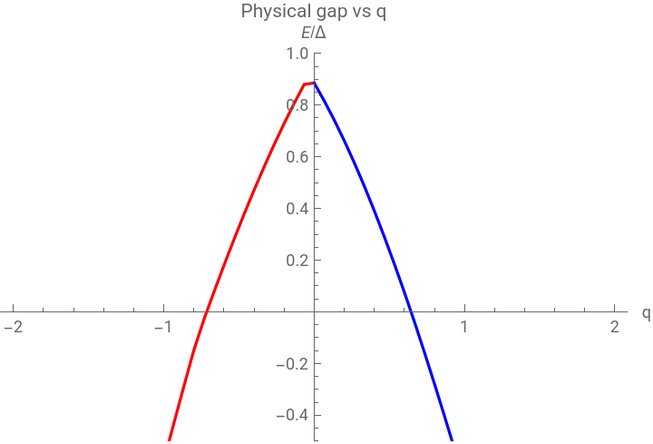


Zeros for q > 0
Zeros for q < 0
Printing the results
Collecting the zeros and sorting with increasing absolute value
First two zeros with smaller absolute value that corresponds to the physical opposite momenta at which the gap closes
Definition of quality factor for the rectification of supercurrent
η density plot
η density plot
Parameters setting
Function for the calculation of the rectification coefficient as a function of two parameters
Axis ranges for the two parameters of the density plot
Collecting the data in a matrix
Saving the data
Importing the data for the plot
Extraction of the rectification coefficient (in order to get the q - values at which gap cloles the procedure is analogue)
Points for the density plot
Color map
Color map
Mapping the colormap to the points
Function that eliminates .0 after the integers
Generating ticks in LaTeX font with cleanNumber
Plot with legend
CITE THIS NOTEBOOK
CITE THIS NOTEBOOK
Intrinsic and tunable superconducting diode effect in quantum spin hall systems
by Samuele Fracassi, Simone Traverso, Stefan Heun, Maura Sassetti, Matteo Carrega, Niccolo Traverso Ziani
Wolfram Community, STAFF PICKS, January 30, 2026
https://community.wolfram.com/groups/-/m/t/3631500
by Samuele Fracassi, Simone Traverso, Stefan Heun, Maura Sassetti, Matteo Carrega, Niccolo Traverso Ziani
Wolfram Community, STAFF PICKS, January 30, 2026
https://community.wolfram.com/groups/-/m/t/3631500