The RadiaCode is a USB / Bluetooth gamma-ray spectrometer the size of a deck of cards: a 1 cm³ CsI(Tl) scintillator coupled to a silicon photo-multiplier, with on-board pulse-height analysis into 1024 channels. The phone app shows the live spectrum and tries to identify the radioisotopes you are pointing at. This post walks through doing the same thing — and considerably more — in the Wolfram Language, with an open-source toolkit that imports the device's native files, plots calibrated spectra, finds photopeaks, fits Gaussians, and ranks candidate isotopes against a built-in gamma-line library. All of the code below runs offline against a handful of sample files included with the toolkit, so you can reproduce everything without owning a detector.
By the end you will have: (a) a calibrated, log-scale spectrum plot of an Am-241 disc source, (b) an energy-resolution measurement at 60 keV and at 583 keV, (c) a ranked list of candidate isotopes for a thorium sample, and (d) a dose-rate map of a survey route plus a time-frequency spectrogram of a long potassium-40 measurement. Every claim is backed by a plot.
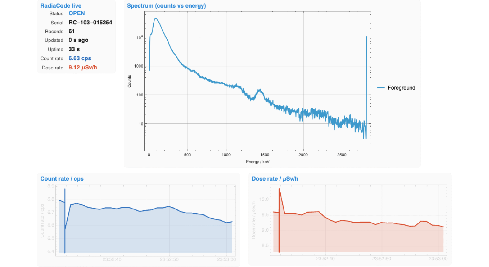
Below: a 60-frame screen recording of the live-updating dashboard built with this toolkit, captured from a connected RadiaCode-103 (serial RC-103-015254) over 97 s of acquisition. The spectrum panel rebuilds as fresh records arrive; the count-rate and dose-rate panels scroll the corresponding traces; the status block at the top-left shows the latest values. The dashboard is just a Dynamic[] expression depending on a state Association the toolkit keeps fresh in the background — no event loop in user code.
Installation
Installation
Three install paths, in order of effort. All three give you the same offline analysis API; only B and C add the ability to talk to a connected detector.
A. Single-file bundle (offline analysis only)
A. Single-file bundle (offline analysis only)
If you just want to read RadiaCode files, fit calibrations, plot spectra, find peaks, identify isotopes, and play with the survey data: this is all you need. Download one file and Get it. No clone, no Python, no compilation. Reproduces every cell of this notebook.
Download `RadiaCodeToolsBundle.wl` from the repo (https://github.com/mthiel74/radiacode-wolfram/blob/main/Wolfram/RadiaCodeTools/RadiaCodeToolsBundle.wl) or directly from this Community post, then:
In[]:=
(*Editthepathtomatchwhereyousavedthebundle.Defaultfindsitnexttothenotebook(thelayoutusedwhenyoudownloadthepost'sattachmentstogether),andfallsbacktotherepo'smastercopyifyouhappentobeevaluatinginaclone.*)$bundle=NotebookDirectory[]<>"RadiaCodeToolsBundle.wl";If[!FileExistsQ[ExpandFileName[$bundle]],$bundle=FileNameJoin[{NotebookDirectory[],"..","RadiaCodeTools","RadiaCodeToolsBundle.wl"}]];Get[ExpandFileName[$bundle]]
The bundle is the concatenation of every package file under `Wolfram/RadiaCodeTools/` in load order — roughly 3,600 lines of Wolfram Language defining ~70 public functions. Sample data files referenced below (data_am241.xml, data_th232_plus_background.xml, trinitite.xml, K40.rcspg) live in the repo's tests/data/ directory (and are bundled into community/data/ for direct download); grab them alongside the bundle if you want to evaluate this notebook end-to-end.
B. Python bridge (live device, easiest live install)
B. Python bridge (live device, easiest live install)
If you have a RadiaCode plugged in via USB and want live acquisition: pair the bundle (or a clone of the repo) with the upstream Python tools that drive the device. This is the path of least resistance because the protocol decoder is already written and maintained. Setup:
In[]:=
(*inashell,notinMathematica*)(*gitclonehttps://github.com/mthiel74/radiacode-wolfram*)(*cdradiacode-tools&&pipinstallradiacode*)
Then from Mathematica, after `Get["...init.wl"]` (or the bundle), the Device.wl namespace is available. It auto-detects your python3 even if the Mathematica front-end's PATH is stripped (it probes ~/anaconda3, /opt/homebrew, etc.):
In[]:=
(*RadiaCodeTools`Device`RadiaCodeDevices[]*)(*spec=RadiaCodeTools`Device`RadiaCodeAcquire[*)(*"AccumulationTime"->Quantity[60,"Seconds"]];*)(*RadiaCodeTools`SpectrumPlot`RCSpectrumPlot[spec]*)
C. Pure-Wolfram native via libusb (no Python at runtime)
C. Pure-Wolfram native via libusb (no Python at runtime)
If you would rather not have Python in your runtime, the toolkit ships a LibraryLink shim that talks to the device directly through libusb. Same Wolfram-native API as Option B, completely self-contained at runtime. One-time setup is a shell-command-then-wolframscript dance:
In[]:=
(*inashell*)(*brewinstalllibusb*)(*gitclonehttps://github.com/mthiel74/radiacode-wolfram*)(*cdradiacode-tools*)(*wolframscript-fileWolfram/RadiaCodeTools/clib/build.wls*)
After the build step a `radiacode_link.dylib` (or .so on Linux) appears next to the C source. The package then loads it transparently:
In[]:=
(*RadiaCodeTools`DeviceNative`RadiaCodeNativeDevices[]*)(*h=RadiaCodeTools`DeviceNative`RadiaCodeNativeOpen[]*)(*RadiaCodeTools`DeviceNative`RadiaCodeNativeReadSpectrum[h]*)(*RadiaCodeTools`DeviceNative`RadiaCodeNativeClose[h]*)
Implementation note: the RadiaCode is a vendor-class USB device with bulk endpoints (0x01/0x81), not a HID device. hidapi's `hid_enumerate` returns nothing for it; you need libusb. Verified on macOS against an attached RC-103: byte-identical spectrum payload to the Python bridge, with no Python in the process tree.
The rest of this post
The rest of this post
Everything below assumes you have one of the three options loaded. We use sample data shipped with the repo so the notebook evaluates with no detector attached, which is what the bundle alone gets you. If you have a detector and prefer live acquisition, substitute `RadiaCodeAcquire[...]` or `RadiaCodeNativeReadSpectrum[h]` for the `ImportRCSpectrum[file]` calls below — the rest of the pipeline is identical.
1. The detector and the toolkit
1. The detector and the toolkit
The RadiaCode-10x family (Scan-Electronics, RU) behaves as a vendor-class USB device with bulk endpoints (0x01 / 0x81) on the host side; on the air it also speaks Bluetooth Low Energy. Internally it is a CsI(Tl) crystal read out by a 6 × 6 mm² SensL SiPM, with a Hamamatsu-style charge-integrating front end and a 12-bit ADC binning into 1024 channels. Photon energy maps to channel by a quadratic calibration, E(c) = a₀ + a₁ c + a₂ c², stored in the device's flash and exported with every spectrum.
The companion phone / Windows app saves spectra as an XML file that contains the cumulative channel counts, the calibration coefficients, the elapsed acquisition time, and (optionally) a background spectrum collected separately. Because every interesting piece of physics is in that XML, post-processing in a language like Wolfram is straightforward.
RadiaCodeTools (https://github.com/mthiel74/radiacode-tools) is an idiomatic Wolfram Language port of the upstream Python tools. It exposes a flat namespace of functions — no GUI required — that turn the device's files into Associations and Datasets ready for Query, Plot, NonlinearModelFit, GeoListPlot, ArrayPlot, etc.
Sample data files (a few small .xml / .rcspg samples used by the worked examples below) ship alongside the post in a `data/` subfolder. If you cloned the repo instead, they live at `tests/data/`. This cell tries both:
In[]:=
$dataDir=SelectFirst[{FileNameJoin[{NotebookDirectory[],"data"}],NotebookDirectory[],FileNameJoin[{NotebookDirectory[],"..","..","tests","data"}]},DirectoryQ];{"$dataDir"->$dataDir,"contents"->(FileNames["*.xml"|"*.rctrk"|"*.rcspg"|"*.n42",$dataDir]//Map[FileNameTake]//Sort)}
Out[]=
{$dataDir/Users/thiel/GitHub/radiacode-wolfram/Wolfram/community/data,contents{data_am241.xml,data_th232_plus_background.xml,K40.rcspg,trinitite.xml}}
About the detector — two infographics
About the detector — two infographics
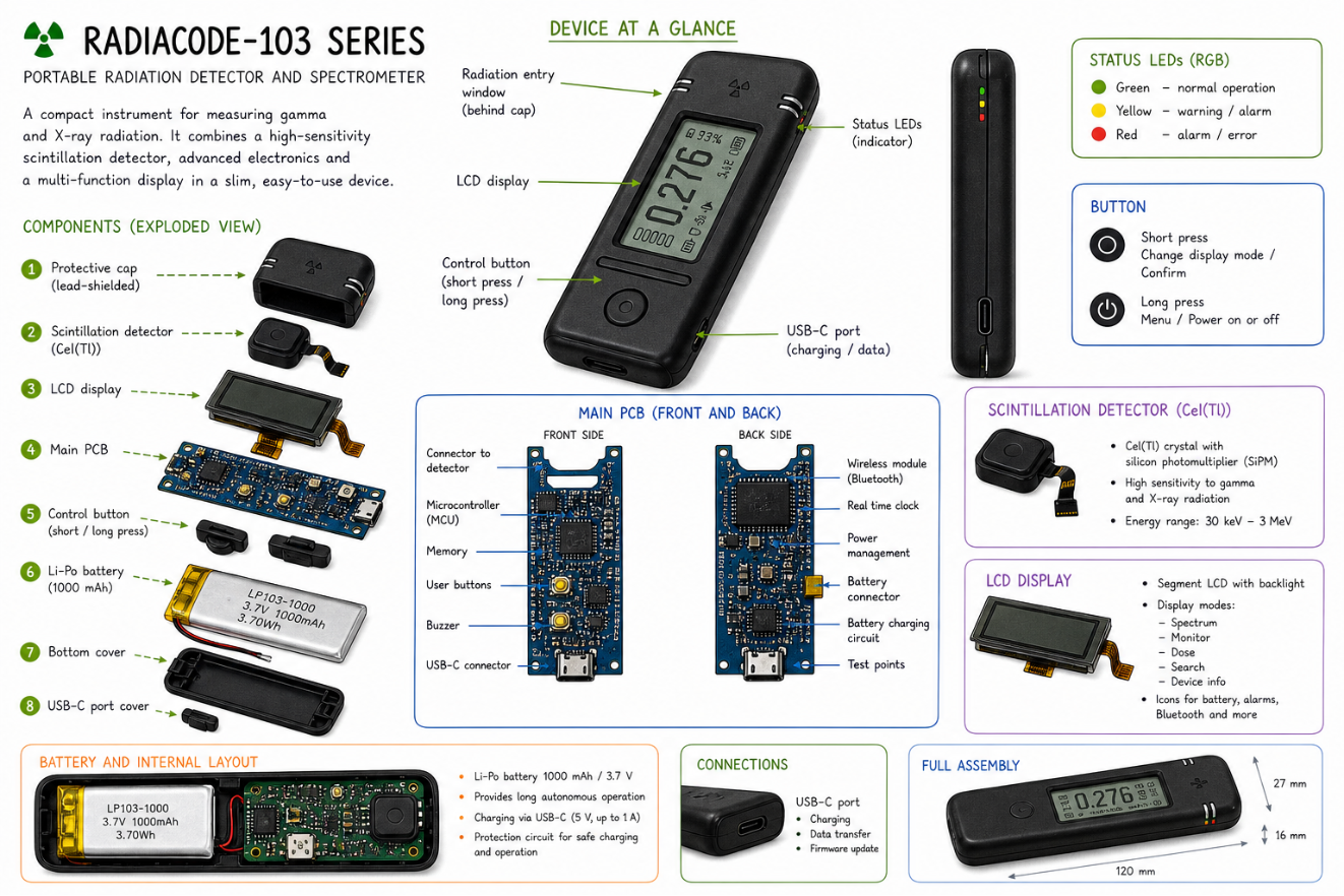
Two reference figures before we start. Both were generated with OpenAI's GPT image-generation model from a verbal prompt and a few photos of the device, so treat them as illustrative summaries rather than authoritative engineering drawings (the official RadiaCode-100 series page “radiacode.com/100-series” and the manufacturer's knowledge base “radiacode.com/knowledge” are the canonical source). Click either image to open the full-resolution copy in a new browser tab from Wolfram Cloud.
1. Components and physical layout. Click the image (or this link) for the full-resolution copy: wolframcloud.com/obj/m.thiel/radiacode_teardown.png
2. How the scintillation detector works. Click the image (or this link) for the full-resolution copy: wolframcloud.com/obj/m.thiel/radiacode_howitworks.png
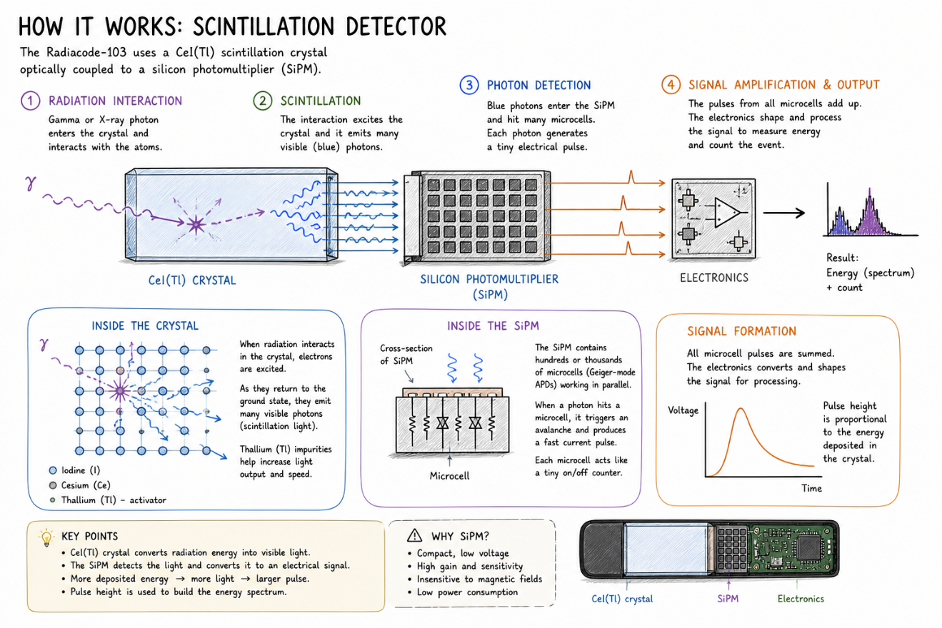
Both infographics were produced by GPT image generation (OpenAI) and uploaded to Wolfram Cloud via `CloudPublish[Import[path], Permissions -> "Public"]`. The links above point at those public CloudObjects. Acknowledgement: the GPT prompts referenced the manufacturer's published photos and product descriptions for visual reference.
2. The physics in three paragraphs
2. The physics in three paragraphs
A gamma photon entering the CsI(Tl) crystal deposits some or all of its energy via photo-electric absorption, Compton scattering, or (above 1.022 MeV) pair production. The deposited energy creates electron-hole pairs in the CsI host (∼15 eV per pair, the empirical pair-creation energy in CsI(Tl)); those carriers transfer their energy to thallium activator sites, which de-excite by emitting visible photons centred around 550 nm. The SiPM converts those photons into a charge pulse whose integrated area is proportional to the deposited energy. Pulses are histogrammed channel-by-channel; photopeaks appear at energies where the full photon energy was absorbed in a single interaction.
Identifying isotopes from a spectrum means matching the locations of photopeaks to the characteristic gamma lines of candidate nuclides. The trick is that one peak is rarely diagnostic: a 1460 keV line could be K-40 (1461 keV, the dominant natural-background line) or the Compton edge of Tl-208's 2614 keV emission feeding counts into that energy region; a faint 122 keV peak could be Co-57, Eu-152, or a Th-232 daughter. The function we build below scores candidates by a peak-weighted match: candidates whose expected lines coincide with the strongest observed peaks rise to the top.
3. Reading and plotting a spectrum
3. Reading and plotting a spectrum
Start with an easy case: an Am-241 calibration disc. The radioactive isotope sits in most household smoke detectors and emits a single strong gamma at 59.5 keV (plus a few low-intensity lines we will ignore). The XML file records 613 s of acquisition.
The cumulative counts vector is what we plot. RCSpectrumPlot applies the polynomial calibration so the x-axis is in keV; the y-axis is logarithmic by default because the dynamic range of an even modestly active source spans four decades.
The 60 keV photopeak dominates everything else. The shoulder to its left is partly Compton scattering inside the crystal and partly the L-shell X-ray escape peak (∼34 keV below the photopeak). PeakChannels lists the n highest-count bins with their calibrated energies.
4. Finding photopeaks programmatically
4. Finding photopeaks programmatically
PeakChannels just picks the top-n bins by raw count, which is fine for a clean source but useless for a busy spectrum: adjacent bins on the same peak crowd out everything else. FindPhotopeaks (in the new Spectroscopy package) does proper local-maximum detection with a moving-average detrending step and a non-maximum suppression window.
Run the same thing on the Th-232 sample (with its background spectrum subtracted in the parser). Thorium's natural-decay chain emits dozens of gammas; the strongest visible ones are Pb-212 at 238 keV, Tl-208 at 583 keV and 2614 keV, Ac-228 around 911-968 keV, and Bi-214 at 609 keV (Ra-226 series, present from ambient soil).
Useful sanity check: overlay the located peak energies onto the spectrum. Vertical red lines mark each FindPhotopeaks pick; the strongest ones land squarely on the K-X-ray, Pb-212 238 keV, Tl-208 583 keV / Bi-214 609 keV doublet, and Ac-228 911 keV groups.
5. Energy resolution: fitting a Gaussian to a peak
5. Energy resolution: fitting a Gaussian to a peak
Visualise the fit. PlotPeakFit overlays the data points and fitted curve on the same axes and labels the panel with the FWHM/E result — one line of code instead of a Module of plumbing.
8–9 % at 583 keV is right in the published CsI(Tl) band, and ∼30 % at 60 keV is similarly typical for a small inorganic scintillator at that energy: the L X-ray escape shoulder dominates the line shape and the calibration polynomial itself starts to lose precision at the low end. A user wanting cleaner low-energy resolution would refit the calibration with more low-energy lines (Calibrate.wl in the toolkit does that).
6. The phone-app feature: identifying isotopes
6. The phone-app feature: identifying isotopes
The new IdentifyIsotopes function compares the FindPhotopeaks output against a built-in library of common gamma-emitting isotopes (Am-241, Cs-137, Co-60, K-40, Na-22, Ba-133, Eu-152, Mn-54, Co-57, plus the dominant Bi-214 / Pb-214 (Ra-226 series) and Tl-208 / Ac-228 / Pb-212 (Th-232 series) lines). Each library entry is {energy, branching ratio}. Scoring works in two stages:
(1) For each library line within the user-chosen energy tolerance of an observed peak, mark the line as matched and note its branching intensity. (2) Sum the matched intensities weighted by the height of the peak they matched (relative to the single strongest peak). This is the "PeakWeight" column. The plain "Score" column is the unweighted fraction of the isotope's characteristic lines that were seen at all.
Run the identifier on Am-241 first. The expected answer is Am-241, with a single matched line at 59.5 keV and a high PeakWeight (the matched line is the dominant peak in the spectrum).
And on the Th-232 sample. Members of the Th decay chain (Pb-212, Ac-228, Tl-208) and the co-present Ra-226 chain (Bi-214, Pb-214) should rise to the top. No single isotope is the answer here — thorium-bearing samples in equilibrium emit a dozen lines from a dozen daughters.
7. A historical sample: trinitite
7. A historical sample: trinitite
Trinitite is the green glass formed when desert sand at the Trinity test site (New Mexico, July 1945) was fused by the world's first nuclear detonation. A trinitite specimen retains traces of the device's plutonium fuel (and therefore Am-241 from Pu-241 decay), Cs-137 fission product, and the neutron-activated soil constituents.
Source: trinitite.xml is a sample file shipped with the upstream Python toolkit (github.com/ckuethe/radiacode-tools), contributed by a hobbyist who measured a trinitite chip with their own RadiaCode for ~72 h. We are reusing that measurement here because (a) trinitite is a charismatic test case and (b) almost no reader will have a piece on hand. Substitute your own ImportRCSpectrum[...] for any sample you have measured yourself.
Am-241 lights up because Pu-241 in the fission fuel beta-decays to Am-241 with a 14.3 yr half-life; eight decades on (∼5.6 half-lives) essentially all the original Pu-241 has converted to Am-241 (>98 %). Cs-137 is a primary fission product (∼6 % yield from U-235 fission, 30.1 yr half-life). Eu-152 is the giveaway of neutron activation — 13.5 yr half-life, formed by Eu-151(n,γ) on natural europium in the soil. This is exactly the cocktail one expects from a 1945 implosion device's calling card.
We can also fit the trinitite 60 keV Am-241 peak and overlay the result on the data. Acquisition time alone does not change a detector's intrinsic resolution — FWHM/E is set by the crystal physics — but a long run reduces statistical scatter and makes the photopeak shape more obvious against the Compton continuum, which is what the visualisation lets you see:
8. Survey mode: dose rate along a track
8. Survey mode: dose rate along a track
RadiaCode also logs GPS position, ambient dose rate, and count rate during a field survey and writes them to a .rctrk file. Each point is timestamped and tagged with the device's reported accuracy in metres.
Note: the route below is a SIMULATION, not a real RadiaCode recording. The author of this post has not yet captured a survey walk with their own detector; rather than reuse the upstream toolkit's synthetic test fixture (which clusters 223 points within ∼100 m of the (0°, 0°) origin in the Gulf of Guinea), we synthesise something legible here:
• The path is a real walking route through central Berlin obtained from `TravelDirections`, so the polyline follows actual streets;
• Each polyline vertex gets a fake timestamp, accuracy, count rate and dose rate, with a deliberately injected hot-spot segment near the eastern end of the route.
The plotting / filtering / histogram pipeline is identical for a real recording — swap the synthetic Association below for `RadiaCodeTools`Formats`ImportRCTrack[yourFile.rctrk]` and the rest of this section works unchanged.
• The path is a real walking route through central Berlin obtained from `TravelDirections`, so the polyline follows actual streets;
• Each polyline vertex gets a fake timestamp, accuracy, count rate and dose rate, with a deliberately injected hot-spot segment near the eastern end of the route.
The plotting / filtering / histogram pipeline is identical for a real recording — swap the synthetic Association below for `RadiaCodeTools`Formats`ImportRCTrack[yourFile.rctrk]` and the rest of this section works unchanged.
RCTrackPlot drops the points onto a Wolfram GeoListPlot, coloured by dose rate. Because the underlying coordinates came from `TravelDirections`, the polyline follows real Berlin streets — Pariser Platz, Unter den Linden, Karl-Liebknecht-Straße — rather than cutting across blocks. The injected hot-spot segment shows up as the warm-coloured stretch near the Alexanderplatz end.
The dose-rate histogram cleanly separates the two populations: the bulk-of-route background near 0.10-0.13 μSv/h, and the spike near 0.55-0.65 μSv/h from the hot-spot leg. On a real survey the shape is typically log-normal around background with a long tail of hot points wherever the detector paused near elevated activity.
9. Time-frequency view: the K-40 spectrogram
9. Time-frequency view: the K-40 spectrogram
A spectrogram is a 2-D matrix indexed by time and channel: each row is one short spectrum, each column is one channel. Plotted as a heatmap it shows you which energies show up steadily (natural background, a fixed source) and which come and go (a sample brought close, then taken away). The K40.rcspg file is a long unattended measurement focused on the 1461 keV K-40 line in a few kilograms of potassium chloride salt.
The bright vertical band near channel ∼560 (which the calibration places at ∼1461 keV) is the K-40 photopeak; horizontal striations mark times when the count rate dropped (the operator stepped away). Collapsing the matrix along the time axis gives a single integrated spectrum we can run through the same FindPhotopeaks / IdentifyIsotopes pipeline.
Each spectrogram row is the *delta* counts since the previous sample, and the file's `HistoricalSpectrum` field is the device's accumulated counts from before the recording started. Here that historical baseline is a long calibration run from a different session without the K-40 sample, so summing it in would swamp the real signal. We collapse only the delta rows to recover the spectrum acquired during this recording:
And the resolution at the K-40 1461 keV line. At this energy CsI(Tl) is approaching the Poisson limit, so we expect about 5–6 % FWHM/E:
10. Live acquisition: an interactive dashboard
10. Live acquisition: an interactive dashboard
This is the headline feature of the toolkit: the same Wolfram Language code that imports an XML file can talk to the device itself. With a RadiaCode plugged in over USB, the cells in this section read live spectra, count rates, and dose rates straight from the detector and feed them into a self-updating Dynamic[] dashboard — exactly the screen recording shown at the top of the post. The rest of this section walks through how the dashboard is built, what its API looks like, and how to read it.
How it is wired up
How it is wired up
Three pieces compose: a producer that talks to the device, a consumer that turns each ndjson record into Wolfram state, and a Dynamic[] expression that re-renders whenever the state changes.
• Producer. Either the upstream Python `rcmultispg.py --stdout` (Option B in the Installation section) or the native LibraryLink + libusb shim (Option C) emits one JSON record per poll: spectrum samples (cumulative counts + calibration), realtime samples (count rate, dose rate, charge, temperature), and GPS samples if available.
• Consumer. `LiveViewer.wl` tails that stream into a per-session state Association: latest spectrum, a sliding window of realtime samples, GPS history, status fields. A ScheduledTask polls the buffer every ∼0.5 s, parses any new lines, and updates the state. No explicit event loop in user code.
• Display. `RadiaCodeDashboard[streamId]` returns `Dynamic[Refresh[buildDashboard[streamId], UpdateInterval -> 1, TrackedSymbols :> {}]]`. The Refresh ticks once a second, buildDashboard reads the current state Association and lays out four panels (status block, spectrum, count-rate trace, dose-rate trace), and the front-end re-renders. That is the entirety of the reactivity story — no manipulators, no observer pattern, just one Dynamic[].
• Producer. Either the upstream Python `rcmultispg.py --stdout` (Option B in the Installation section) or the native LibraryLink + libusb shim (Option C) emits one JSON record per poll: spectrum samples (cumulative counts + calibration), realtime samples (count rate, dose rate, charge, temperature), and GPS samples if available.
• Consumer. `LiveViewer.wl` tails that stream into a per-session state Association: latest spectrum, a sliding window of realtime samples, GPS history, status fields. A ScheduledTask polls the buffer every ∼0.5 s, parses any new lines, and updates the state. No explicit event loop in user code.
• Display. `RadiaCodeDashboard[streamId]` returns `Dynamic[Refresh[buildDashboard[streamId], UpdateInterval -> 1, TrackedSymbols :> {}]]`. The Refresh ticks once a second, buildDashboard reads the current state Association and lays out four panels (status block, spectrum, count-rate trace, dose-rate trace), and the front-end re-renders. That is the entirety of the reactivity story — no manipulators, no observer pattern, just one Dynamic[].
Reading the dashboard
Reading the dashboard
Looking at the hook video at the top of the post:
• Top-left status block. Status (open/closed), serial, record count, time since last update, uptime since you called RadiaCodeStream[], the latest count rate in cool blue, the latest dose rate in warm red. These are pulled fresh from the state Association on every Refresh tick.
• Spectrum panel. The cumulative photopeak histogram, log-scaled counts vs calibrated keV. It looks essentially static through a short recording because each new spectrum sample adds only a tiny correction to the cumulative counts — that is by design; the shape stabilises with integration time.
• Count-rate trace (blue, lower-left). Wall-time series, filled-area undertone, ~1 sample/s on this device. A trend down means the operator is moving away from a source; a spike usually means a stationary measurement next to something hot.
• Dose-rate trace (red, lower-right). Same axis convention but in μSv/h (the producer reports Sv/h; the dashboard multiplies by 10ü to keep the y-axis legible).
• Top-left status block. Status (open/closed), serial, record count, time since last update, uptime since you called RadiaCodeStream[], the latest count rate in cool blue, the latest dose rate in warm red. These are pulled fresh from the state Association on every Refresh tick.
• Spectrum panel. The cumulative photopeak histogram, log-scaled counts vs calibrated keV. It looks essentially static through a short recording because each new spectrum sample adds only a tiny correction to the cumulative counts — that is by design; the shape stabilises with integration time.
• Count-rate trace (blue, lower-left). Wall-time series, filled-area undertone, ~1 sample/s on this device. A trend down means the operator is moving away from a source; a spike usually means a stationary measurement next to something hot.
• Dose-rate trace (red, lower-right). Same axis convention but in μSv/h (the producer reports Sv/h; the dashboard multiplies by 10ü to keep the y-axis legible).
The complete API — live
The complete API — live
These are the only four calls you need. THE CELLS ARE LIVE — when you evaluate them with a RadiaCode plugged in over USB they actually open a stream, render the live dashboard, and poll the device. If no detector is attached they return a Failure[…] you can read for the reason; nothing else in the notebook breaks.
First a sanity check: the toolkit reports the serial numbers of every attached RadiaCode. An empty list means no device detected; a Failure[…] usually means the radiacode Python package is not installed on the right interpreter (Option B in the Installation section) or the libusb shim has not been compiled (Option C). See `Notebooks/LiveDashboard.nb` for a diagnostics notebook that resolves both.
Open the stream. PollingInterval is how often the producer asks the device for a fresh spectrum, in seconds; realtime samples arrive at ∼1 Hz independent of this setting. Returns a stream id you pass to the other API calls.
Render the dashboard. Returns a Dynamic[] that self-updates in place every second; spectrum, count-rate trace, and dose-rate trace all rebind as fresh records arrive. Evaluate this cell once and watch the live recording unfold inside the notebook.
Pull the current state at any time as a plain Association — handy for ad-hoc analysis, snapshotting, or saving. Re-evaluate to get a fresh snapshot of whatever the stream looked like the moment you ran the cell.
A ready-to-run version of this section, with a pre-flight diagnostics cell that prints the resolved Python path, repo root, and verifies that the radiacode package imports, ships in `Notebooks/LiveDashboard.nb`.
Stopping the stream
Stopping the stream
When you are done, free the device by evaluating the close call. The cell below is wrapped in a Wolfram comment so that an "Evaluate Notebook" sweep does NOT inadvertently tear the stream down before any data has flowed (which would leave the dashboard above stuck on CLOSED / 0 records). When you actually want to stop, remove the leading `(*` and trailing `*)` and evaluate the cell.
11. Discussion and future directions
11. Discussion and future directions
What we have built reproduces the RadiaCode phone app's two headline features — live spectrum and isotope hint — in a few hundred lines of Wolfram Language, plus a proper resolution measurement the phone app does not give you, plus GeoListPlot of dose rate, plus a time-frequency spectrogram. The pieces compose: every function takes the same Association the file parser returns, so swapping in your own spectrum (drop a .xml on the path and call ImportRCSpectrum) is a one-line change.
Several natural extensions are not in the toolkit yet but are each one notebook away:
● Background subtraction with χ² goodness-of-fit — given a separately-measured background, scale and subtract it under the foreground and report the residual sum of squares. RCSpectrumPlot already supports "Background" -> "Subtract"; what is missing is the χ² diagnostic.
● Activity estimation in becquerels — given an efficiency curve ϵ(E) for the detector geometry, the area under a fitted photopeak divided by ϵ(E) × (branching ratio) × (live time) gives the source activity. FitGaussianPeak already exposes A and σ; the missing piece is the efficiency curve itself, which the toolkit's Calibrate.wl could absorb if the user provided a known-activity calibration source.
● Compton continuum modelling — subtracting the analytic Klein-Nishina continuum from a peak fit removes the linear-baseline assumption that breaks down at high energies and improves resolution estimates in busy spectra.
● Cross-correlation of multiple spectra to flag anomalies — given a library of "normal" backgrounds (your house, your car, your office), the residual after best-matched scaled subtraction is a cheap and cheerful anomaly detector.
● Confidence intervals on the identification ranking — bootstrap the FindPhotopeaks pass over Poisson-resampled counts and report the rank distribution of each candidate. This catches the "Pb-212 vs Bi-214 vs Pb-214" sibling-rivalry case that any flat scoring makes hard.
● Isodose contours on the survey map — interpolate the GeoPosition + dose-rate cloud onto a regular grid and contour, the same way a meteorologist contours a temperature field. The Wolfram functions ListInterpolation + ContourPlot do most of the work.
All of the above are, by the toolkit's design, additive. The parser layer is fixed; the analysis layer can grow.
References and acknowledgements
References and acknowledgements
● Wolfram port (this toolkit, the bundle, the Spectroscopy / Calibrate / LiveViewer packages, the LibraryLink + libusb shim, the test suite, and this post) — https://github.com/mthiel74/radiacode-wolfram (MIT).
● Upstream Python toolkit — Chris Kuethe's radiacode-tools (https://github.com/ckuethe/radiacode-tools, MIT, Copyright (c) 2023 Chris Kuethe). All sample data files used in the worked examples (data_am241.xml, data_th232_plus_background.xml, trinitite.xml, K40.rcspg, plus the unused walk.rctrk / xray.ndjson / deadtime triplets shipped with the source repo) come from there and are redistributed under MIT with attribution. The Wolfram port also draws on Chris's file format definitions, deadtime semantics, and N42 conversion conventions — thanks!
● Underlying device protocol — Maxim Andreev's `radiacode` Python library (https://github.com/cdump/radiacode), MIT, which speaks the RadiaCode USB / Bluetooth protocol; both the Python bridge (Option B in Installation) and the libusb LibraryLink shim (Option C) follow the protocol it documents.
● Knoll, G. F. "Radiation Detection and Measurement", 4th ed. Wiley, 2010. Chapters 8–10 cover scintillator physics, the photopeak / Compton anatomy of a gamma spectrum, and the FWHM/E figure of merit.
● Brookhaven National Laboratory ENSDF (Evaluated Nuclear Structure Data File) — https://www.nndc.bnl.gov/ensdf/ — authoritative source for the gamma-line energies and branching ratios in the built-in IsotopeLibrary; the Lund/LBNL Table of Isotopes (https://nucleardata.nuclear.lu.se/toi/) is a useful searchable mirror.
● IAEA Nuclear Data Sheets — https://www.iaea.org/resources/databases/nuclear-data-sheets Authoritative cross-check for individual decay schemes.
● This notebook is regenerated from Wolfram/community/build_RadiaCodeSpectroscopy.wls; the .nb is a build artefact. Tests for the underlying functions live in Wolfram/Tests/Spectroscopy.wlt.
CITE THIS NOTEBOOK
CITE THIS NOTEBOOK
Gamma spectroscopy with the RadiaCode detector
by Marco Thiel
Wolfram Community, STAFF PICKS, May 3, 2026
https://community.wolfram.com/groups/-/m/t/3710670
by Marco Thiel
Wolfram Community, STAFF PICKS, May 3, 2026
https://community.wolfram.com/groups/-/m/t/3710670