In this computational essay, I will explore Principal Component Analysis (PCA) to understand its role as a dimensionality reduction technique. I will implement PCA from scratch on the MNIST dataset and demonstrate its connection to fundamental linear algebra concepts, including matrix diagonalization and singular value decomposition. For an in-depth mathematical exploration, please refer to my computational essay Linear Algebra Meets Data Science in PCA.
Introduction
High-dimensional data is often quite cumbersome to work with, both computationally and analytically. This is due to challenges such as increased computational cost, difficulty in visualization, and the sparsity of data in high-dimensional spaces. As a result, we often seek to extract a latent lower-dimensional structure that captures the essential patterns hidden within the redundant and noisy high-dimensional data.
Principal Component Analysis (PCA) is a widely used algorithm for dimensionality reduction. It constructs a lower-dimensional representation of a large dataset while preserving as much of the information contained in the original data. As we will see, what “keeping as much information as possible” practically means is to find the directions--called principal components--along which the greatest variance is captured.
Succinctly summarized, the main objective of PCA is “to find the projections of sample data points ∈ onto a lower-dimensional subspace while retaining as much variance in the original data.”
n
x
i
d
R
Datasets
To demonstrate the implementation of PCA, I will use the Iris dataset. The Iris dataset is a small classic dataset from Fisher, 1936. It is one of the earliest datasets used for evaluating classification methods. The data set contains 3 classes of 50 instances each, where each class refers to a type of iris plant. There are four features for each data point.
In[]:=
datasetIrises=ResourceData[ResourceObject["Sample Data: Fisher's Irises"]]
Out[]=


Data Structures and Notations
Data Matrix
Data Matrix
In PCA, we consider a dataset of observations, which is essentially data matrix where is the size of the sample and is the number of features or variables
nd
X
n
d
So, from the Iris dataset, we create our data matrix containing the 150 data points.
X
In[]:=
X=#[[2]][[1]]&/@DeleteCases[#,"Species"->_]&/@Normal[Normal[datasetIrises]];
In[]:=
Dimensions[X]
Out[]=
{150,4}
We have created a matrix in which each data point is represented as a 4-dimensional vector consisting of four features.
1504
Sample Covariance Matrix
Sample Covariance Matrix
Sample covariance matrix plays a very important role in principal component analysis. It is a matrix containing the covariances between the variables.
S
dd
d
It can be shown with mathematics where is the centered data matrix (mean zero).
S
1
n
T
X
c
X
c
X
c
Centered Data Matrix
Centered Data Matrix
First, we compute the sample mean vector
x
In[]:=
x
Out[]=
{5.84333,3.05733,3.758,1.19933}
Then, we compute the centered data matrix by subtracting the mean from each row.
In[]:=
Xc=Subtract[#,]&/@X;
x
Covariance Matrix
Covariance Matrix
Now that we have computed the centered data matrix, we can compute the sample covariance matrix using the formula.
In[]:=
S=1/4*.Xc
Xc
Out[]=
{{25.5421,-1.58067,47.4683,19.2311},{-1.58067,7.07673,-12.2797,-4.53107},{47.4683,-12.2797,116.081,48.2615},{19.2311,-4.53107,48.2615,21.6425}}
Problem Setting
Lower Dimensional Representation
Lower Dimensional Representation
For each data point ∈, our aim is to produce a lower-dimensional representation as a point in ∈ such that . The relationship between our original data points and the lower-dimensional code is described by
x
i
d
R
z
i
k
R
k<d
z
i
T
B
x
i
k
R
where the projection matrix is defined to be an orthogonal matrix .
B
B[,…,]∈
b
1
b
k
dk
R
Now, the question is how we can find the orthonormal vectors that produce the best lower-dimensional representation.
k
Maximum Variance Formulation
Capturing the Largest Variance
Capturing the Largest Variance
As mentioned earlier, the goal of Principal Component Analysis (PCA) is to find a lower-dimensional representation of the original data that retains as much of its information as possible. But what does it mean to “retain information”? In PCA, the information content of the data is quantified by its variance—the degree to which the data is spread out. Therefore, PCA aims to find orthonormal vectors that form a basis for a -dimensional subspace onto which the data can be projected while maximizing the retained variance.
k
k
Variance of the projected data point Tbix
Variance of the projected data point x
T
b
i
If ∈ is a column of the projection matrix , x gives the coordinate of the lower-dimensional projection of in the direction of .
T
b
d
R
B[,…,]
b
1
b
k
T
b
zx
T
B
b
It can be shown that the variance of this coordinate x is Sb where is the sample covariance matrix. This measures how spread the points are in the direction of .
T
b
T
b
S
b
Direction with Maximal Variance
Direction with Maximal Variance
Let us start by finding a single vector that represents the direction in which the variance of the projected data Sb is maximized.
b
T
b
Mathematics show that the maximum value of the variance Sb is the largest eigenvalue of the covariance matrix if we choose the orthonormal vector to be an eigenvector associated with the largest eigenvalue . This eigenvector is known as the first principal component.
T
b
λ
1
b
v
1
λ
1
So, to produce the -dimensional subspace with maximal variance, we can find the largest eigenvalues of the sample covariance matrix . Then, we use the associated eigenvectors to form the projection matrix .
k
k
S
P[,…,]
v
1
v
k
Finding the largest eigenvalues of the Covariance Matrix
k
According to the Spectral Theorem in linear algebra, any symmetric matrix can be decomposed into where with ≥≥…≥ and .
SQΛ
T
Q
ΛDiag(,…,)
λ
1
λ
d
λ
1
λ
2
λ
d
Q(,…,)
v
1
v
d
First, we compute the diagonal matrix with the eigenvalues on its diagonal.
In[]:=
Λ
Out[]=
{{157.502,0.,0.,0.},{0.,9.03949,0.,0.},{0.,0.,2.9133,0.},{0.,0.,0.,0.887857}}
In[]:=
Q=Eigenvectors[S]//Transpose
Out[]=
{{-0.361387,0.656589,0.58203,0.315487},{0.0845225,0.730161,-0.597911,-0.319723},{-0.856671,-0.173373,-0.0762361,-0.479839},{-0.358289,-0.075481,-0.545831,0.753657}}
So, we have successfully decomposed the covariance matrix into .
S
QΛ
T
Q
In[]:=
S==Q..
Λ
Q
Out[]=
True
How to choose
k
One important question in PCA is how to choose .
k
Total and Explained Variance
Total and Explained Variance
Given the sample covariance matrix, there are two important quantities concerning the variance of our data.
1. Total Variance is the sum of the variance in all directions, which corresponds to the trace of the covariance matrix.
T
In[]:=
T=Tr[S]
Out[]=
170.343
2. Variance Explained by PCA is the sum of the variance in the directions of the principal components. Each principal component to accounts for (or explains) a fraction of the total variance.
v
1
v
k
λ/T
For example, the first principal component explains the largest fraction /T of the total variance, and the next principal component explains the next largest fraction /T.
v
1
λ
1
v
2
λ
2
Effective Rank and Scree Plot
Effective Rank and Scree Plot
PCA finds the “true signal” in the redundant and noisy high-dimensional data. Our question is “at which point does the noise obscure the true signal in the data?”
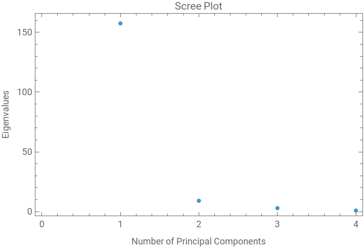
The effective rank is the number of eigenvalues of above the point where noise exceeds the true signal in the data. In other words, the eigenvalues below the effective rank do not contribute much to the explained variance because they are associated with the noise rather than the true signal. Therefore, when choosing , we look for the point where a sudden dropoff in the eigenvalues occurs, which is often visible as an “elbow” in the scree plot.
S
k
The scree plot shows the number of principal components on the horizontal axis and the corresponding eigenvalues on the vertical axis.
k
λ
k
Let us create the scree plot for the Iris dataset.
In[]:=
ListPlot[Eigenvalues[S],PlotLabel->"Scree Plot",Frame->True,FrameLabel->{"Number of Principal Components","Eigenvalues"}]
Out[]=
For comparison, we also create a projection matrix with the last two principal components as columns.
For comparison, we also project the data to the subspace spanned by the last two principal components.
We can see that the three classes are sufficiently spread out when we project the data to the 2-dimensional subspace spanned by the first two principal components.
Conclusion