ABSTRACT (original article): Rather than using the classic models of treating a photon as a particle or a wave, let’s model light by combining the two ideas, and treat light as a simple dipole, a baton-like structure AB whose packet of light (a photon) has shock absorbers at nodes A and B with its energy ensconced between those nodes, where the distance between the nodes is on the order of the photon’s wavelength. With this model the law of reflection follows. So too does Snell’s law of refraction. To do so, as a dipole enters a more dense medium at, say, endpoint B, imagine that B behaves as a tortoise while A behaves as a hare. Such a model implies Fermat’s principle that light follows paths of least time. Furthermore, a law of diffraction surprisingly follows as well. Reasonableness of the model, comparisons with the classic models, and further questions are explored. CITATION (original article): Kothapalli, K. ,Simoson, A. J., Bezuidenhout, G. A. (2023). Light as a Dipole: A Tortoise and Hare Model. In: Sriraman, B. (eds) Handbook of Visual, Experimental and Computational Mathematics. Springer, Cham. https://doi.org/10.1007/978-3-030-93954-0_38-1.
In addition to the original article, allowing a photon also to have an amplitude allows us to view a photon’s propagating path as it dances through space, ricocheting and refracting.
Introduction
Introduction
Is it possible to develop a single elementary model for light that predicts its three-fold phenomena of reflection, refraction, and diffraction? Isaac Newton’s classic particle model when combined with Pierre de Fermat’s assumption that light takes the path of least time predicts reflection and refraction. Christiaan Huygens’s classic wave model predicts diffraction. Combining the two models by rendering the photon as a dipole gives a solution model with respect to the opening question---whose especially satisfying corollary also implies Fermat’s assumption.
The current reigning model of a photon is that it is an electromagnetic wave. As a photon proceeds through space, its time-average electric field strength oscillates, as a veritable bead, with constant frequency along a pole or dipole of fixed length (perpendicular to its propagation). Similarly, its time-average magnetic field strength oscillates along a second pole (perpendicular to the dipole and its propagation) . These two beads trace sinusoidal paths in time and space . Our dipole model ignores the photon’s magnetic field so that a photon is merely the dipole along with its oscillating mean electric field bead. Its endpoint nodes A and B perhaps function as shock absorbers, allowing the photon to tumble as a twirling baton when striking an impermeable surface while its energy is safely stored between its nodes. The figure below shows a dipole AB (as a black vertical pole) at various times (1, 2, and 3) with its electric field bead P tracing a green sinusoidal path with wavelength λ through space and time.
The current reigning model of a photon is that it is an electromagnetic wave. As a photon proceeds through space, its time-average electric field strength oscillates, as a veritable bead, with constant frequency along a pole or dipole of fixed length (perpendicular to its propagation). Similarly, its time-average magnetic field strength oscillates along a second pole (perpendicular to the dipole and its propagation) . These two beads trace sinusoidal paths in time and space . Our dipole model ignores the photon’s magnetic field so that a photon is merely the dipole along with its oscillating mean electric field bead. Its endpoint nodes A and B perhaps function as shock absorbers, allowing the photon to tumble as a twirling baton when striking an impermeable surface while its energy is safely stored between its nodes. The figure below shows a dipole AB (as a black vertical pole) at various times (1, 2, and 3) with its electric field bead P tracing a green sinusoidal path with wavelength λ through space and time.
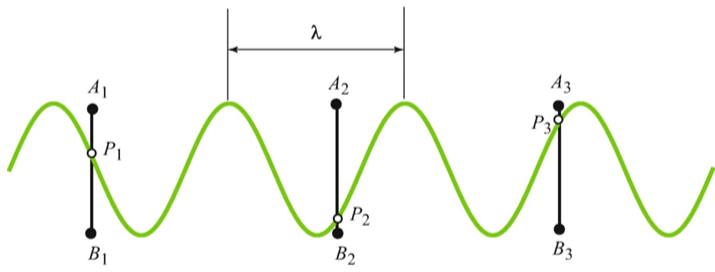
Primitive motion of a dipole
Primitive motion of a dipole
To be more precise, the planar motion of a dipole AB has these properties :
1
.The distance between nodes A and B is constant in time.
2
.The speeds of A and B depend upon the media in which they lie.
3
.The velocities of A and B are ever simultaneously parallel and lie in the plane spanned by the dipole over time.
4
.When striking an obstruction, the incident node of AB instantaneously reverses its velocity, an event called a primitive reflection.
5
. When dipole AB impacts a photon-sensitive screen, it does so at AB’s midpoint.
6
. Paths in which a portion of the interior of dipole AB lies within the interior of impenetrable solids are forbidden.
Reflection
Reflection
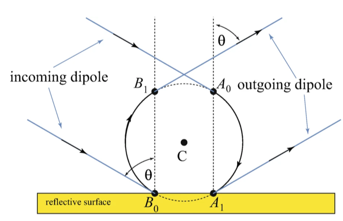
Imagine this scenario: Dipole AB approaches the x-axis, our obstruction, in the x-y plane with constant velocity. By properties 1, 3, and 4, A and B follow parallel paths until, say, B strikes the x-axis, at which point B reverses its path, and the dipole rotates about its midpoint, whereupon A strikes the x-axis, and A reverses its path. By symmetry, A and B proceed along parallel paths in accordance with the six rules above; a reflection has occurred! See the figure below.
To make this argument more precise, let’s transform the rules into equations. With α(t)=(u(t), v(t)), and β(t) =(w(t), z(t)) being the coordinate paths of AB’s nodes in the x-y plane with respect to time t and where d=1 (so that the dipole has unit length), those primitive motion characterizations become
◼
2
(u(t)-w(t))
2
(v(t)-z(t))
◼
2
(u'(t))
2
(v'(t))
2
a
◼
b a
(u'(t),v'(t))=
(w'(t),z'(t)),wherebisB'sspeed,withinitialconditions:
◼
( u(0), v(0) ) = (1, 0) and ( u(0), v(0) ) = (0, 0), a given point in the x-y plane,
◼
(u'(0),v'(0))=
(w'(0),z'(0))=b.
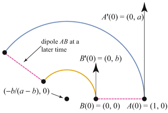
This system of equations, when the product ab is positive---as you might be able to guess---gives the solution paths α(t)= (cos((a - b)t), sin((a - , 0) and β(t)= (cos((a - b)t), sin((a - , 0), namely, concentric circles, as in the figure below.
a
a-b
b)t))-
b
a-b
b
a-b
b)t))-
b
a-b
In Mathematica code, α and β’s interpolating functions can be generated via this command:
In[]:=
NDSolve[{(u'[t])^2+(v'[t])^2==4,(u[t]-w[t])^2+(v[t]-z[t])^2==1,u'[t]==2v'[t],v'[t]==2z'[t],u[0]==1,u'[0]==0,v[0]==0,v'[0]==2,w[0]==0,w'[0]==0,z[0]==0,z'[0]==1},{u,v,w,z},{t,0,15}]
Out[]=
uInterpolatingFunction,vInterpolatingFunction,wInterpolatingFunction,zInterpolatingFunction


When the product ab is negative and a = -b, then the solution a(t) and b(t) are same circle, albeit traced in opposing directions.
An approximation algorithm to solve the above system of equations.
An approximation algorithm to solve the above system of equations.
Let’s adapt Euler’s method for generating approximate solutions for this system of equations. To do so, imagine that node A is a hare, and node B is a tortoise so that a > b > 0. Let Δt be a small positive time increment, and permit the tortoise and hare to dance together so that in Δt time---while the tortoise remains stationary---the hare advances to location P an arc-length distance of a Δ t counter-clockwise along a circular arc of unit radius and center-point Q, the tortoise’s current location. Once the hare arrives at P, allow the tortoise to time-travel back in time by Δt while the hare remains at P. As time repeats itself---with the hare at P---the tortoise advances from Q to R clockwise by bΔt along a circular arc of unit radius and center-point P. Such a hare-tortoise motion over this time-lapse Δt and its déjà vu time-lapse Δt is called a dance step. Thus, to visualize how the tortoise and hare move along, allow them to take n dance steps, where n is some positive integer. The figure below, with n = 3, shows their progress after a lapse of 3Δt, where Δt = 0.3 time units, a = 2, and b = 1.
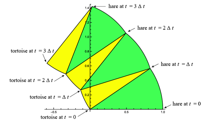
As can be seen in the next figure, as Δt collapses to 0, the trajectories of the tortoise and hare lie along concentric circles, in this case, circles of radii 1 and 2 with center at (-1, 0).
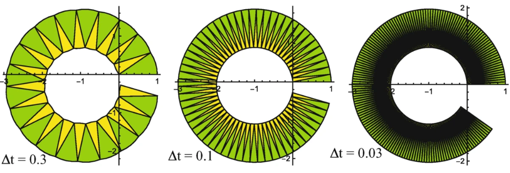
In Mathematica code, here’s a way to generate these figures. The first command angle returns the argument---the angle of orientation with respect to a unit vector in the positive x-direction---of the two-dimensional vector v; the second command sector returns a sector graphic with unit radius given its arc-endpoint, center, central angle, and orientation (clockwise/counterclockwise) as illustrated below. The last command dance generates sequences of sectors, such as the last two figures above.
In[]:=
angle[v_]:=Block[{x=v[[1]],y=v[[2]],w=Pi/2},If[x==0,w=Sign[y]w];(*visa2Dvector*)If[x>0,If[y>=0,w=ArcTan[y/x],w=2Pi+ArcTan[y/x]]];If[x<0,If[y>=0,w=Pi-ArcTan[-y/x],w=Pi+ArcTan[y/x]]];w](*returntheanglebetween0and2Piforv*)sector[X_,O_,w_,c_]:=Block[{q=angle[X-O],g,nX},(*sectorw/centerO,throughX,anglew,clockwise:-1&countercclockwise:1*)nX=O+{Cos[q+cw],Sin[q+cw]};g=Graphics[{If[c==-1,Yellow,Lighter[Green]],Disk[O,1,{q,q+cw}],Black,Circle[O,1,{q,q+cw}],Line[{X,O,O+{Cos[q+cw],Sin[q+cw]}}]},Axes->True];{nX,g}](*returnscoordinateofpointsPorQandgraphicg.*)
Refraction
Refraction
Diffraction
Diffraction
Can the dipole model be coaxed into yielding a diffraction law? As with classic experiments of photons passing through a slit in a non-translucent solid W whose incident surface (except for the slit itself) is a horizontal plane, assume that light waves entering a slit are monochromatic and polarized, so that the wave planes of the photons are all parallel and contain the normal direction to W’s incident plane. Furthermore, the normal to this family of planes is parallel to W’s slit walls, and the slit’s gap is no less than the wavelength λ of the photons.
To implement the dipole model within this framework, consider an x-y plane milieu wherein a flat solid W of thickness h fills the region between y = 0 and y = h, except for a gap---the slit---of width 2 units between x = -1 and x = 1.
Above W and its slit is a photon-sensitive screen along the line y = h + H for some suitable positive distance H. Each photon AB, of constant dipole length 2r with 0 < r < 1, begins its transit-of-the-slit odyssey oriented parallel to and below the x-axis, with node A to the left of node B. Let (p, 0) be the position of AB’s midpoint, its center C, as the dipole reaches the x-axis at time t = 0. See the figure below.
Forbidden zones
Not all photons successfully transit the slit; some crash, which may mean that their energy is absorbed as heat by W; other photons may be reflected at W’s surface along the x-axis, especially so if |p| is much larger than unity. With a little work---see the paper itself---the permissible values of p are those values for which
Dipoles through the slit and onto a screen
Dipoles through the slit and onto a screen
Once dipole AB successfully enters the slit, it continues in the direction of the last primitive reflection . If AB is parallel to the screen just prior to impact, then AB impacts the screen, leaving a mark where AB' s center strikes the screen . If AB fails to be parallel to the screen just prior to impact, it strikes the screen at, say, node A, whereupon node A becomes mired in the screen, which in turn causes AB to rotate about node A; once node B impacts the screen, it too becomes mired, and again a mark is left where AB' s center strikes the screen . That is, in this latter case, if dipole AB initially strikes the screen at point E, then the mark is at E + (r, 0) , (or, if node B struck the screen first, then the mark is at E - (r, 0) ). The figure below shows dipole AB experiencing five reflections and its resultant mark or image on the screen .
Mathematica code to determine dipole screen-impacts for any given permissible p value .
With (p, 0) being the coordinates of a dipole’s center upon dipole entry into a slit of width two units, 2r being the dipole’s length, h being the height of the slit, and y = h + H being the position of a screen, given (p, r, h, H), this code outputs either the x-coordinate s of a dipole’s center with the screen or the Boolean value false if the dipole fails to survive its slit passage.
The user-defined function normalDir returns a vector perpendicular to vector A - B when given the two-dimensional vectors A and B.
The user-defined function solvePt returns the intersection point of the planar lines through points A and B and through points P and Q when given those four planar points.
The user-defined function stepBottom returns the intersection point of a circle with center (p, 0) and radius r with the line x = 1 where 0 < 1 - r < p < 1 and r < h. This output point is where the dipole’s second primitive reflection occurs (on the right-hand wall of the slit).
The user-defined function stepBottom returns the intersection point of a circle with center (p, 0) and radius r with the line x = 1 where 0 < 1 - r < p < 1 and r < h. This output point is where the dipole’s second primitive reflection occurs (on the right-hand wall of the slit).
The user-defined function stepTop returns the intersection point of the circle whose center and radius are center and r, respectively, with the line y = h, where the walls of the slit are at x = ±1.
The user-defined procedure stepNext returns the position V of a dipole on a slit wall after it has ricocheted off the opposite slit wall at node coordinate-position wall, where center is the center of the dipole whose other node has coordinates Q. See Figure \ref{fig:Light_as_a_Dipole_fig32}. Furthermore, P is a vector perpendicular to the direction center - wall; and U gives the coordinates of the dipole’s center at dipole impact point R.
Finally, thruSlit[p, h, r] iterates stepNext, giving the desired output described above.
To generate diffraction patterns similar to the diffraction figure below, collect the outputs s[[1]] from many trials of thruSlit for randomly chosen p values satisfying condition (2). For each even-numbered trial, reverse the sign of non-Boolean s[[1]] values so as to simulate dipole slit-entry at the left-hand wall. Sort this modified list of non-Boolean values into disjoint subintervals or classes of a desired fixed Δ x width on the screen; and plot the relative frequency for each class as a vertical gray-level line segment with x-coordinate being the center of the corresponding subinterval whose gray-level increases with increasing frequency; finally, to allow for dipoles to enter the slit without any slit-wall collisions, plot a black rectangle on the screen with base being the segment -1 + r < x < 1 - r.
To simulate slit experiments of multiple dipoles of a given length, whose p values vary randomly in the permissible zone of Equation (2), p may be taken-- - by symmetry-- - as positive at each new launch n of a dipole, where n is a positive integer . Should that dipole reach the screen with crash site at (q, h + H) , its crash is recorded as q if n is odd, and - q if n is even . The figure below shows a diffraction pattern resulting from the launch of fifty thousand dipoles each of unit length .
To simulate slit experiments of multiple dipoles of a given length, whose p values vary randomly in the permissible zone of Equation (2), p may be taken-- - by symmetry-- - as positive at each new launch n of a dipole, where n is a positive integer . Should that dipole reach the screen with crash site at (q, h + H) , its crash is recorded as q if n is odd, and - q if n is even . The figure below shows a diffraction pattern resulting from the launch of fifty thousand dipoles each of unit length .
Incorporating a photon’s phase in this dipole model
Incorporating a photon’s phase in this dipole model
With a little work---see our original paper---we have
An improved diffraction pattern
An improved diffraction pattern
Step II: Dipole AB’s displacement S from slit-entrance to screen impact. As dipole AB passes through the slit, it experiences several reflections each of which consists of two primitive reflections. Dipole AB’s motion between reflections is Newtonian---that is, linear---and AB’s motion between a reflection’s primitive reflections is Huygensian---that is, rotational. See the figure below.
This dipole model successfully unites light’s three-fold properties of reflection, refraction, and diffraction in an elementary, introductory fashion. Is it anything more than a cute pedagogical tool to help bridge the chasm-like dichotomy between light as a particle and light as a wave, before one goes on to understand the subtle and powerful approach via Maxwell’s equations? We’d like to think so.
CITE THIS NOTEBOOK
CITE THIS NOTEBOOK
Light as a dipole: a tortoise and hare model
by Andrew J. Simoson and Karunakar Kothapalli, King University
Wolfram Community, STAFF PICKS, June 24, 2024
https://community.wolfram.com/groups/-/m/t/3199039
by Andrew J. Simoson and Karunakar Kothapalli, King University
Wolfram Community, STAFF PICKS, June 24, 2024
https://community.wolfram.com/groups/-/m/t/3199039