ABSTRACT (original article): We show that a highly-excited energy eigenfunction () of hydrogen atom can be approximated as an equal-weight superposition of classical elliptic orbits of energy and angular momentum , and component of angular momentum =mℏ. This correspondence is established by comparing the quantum probability distribution and the classical probability distribution () of an ensemble of such orbits. This finding illustrates a general principle: in the semi-classical limit, an energy eigenstate of a quantum system is in general reduced to a collection of classical orbits, rather than a single classical orbit. In light of this quantum-classical correspondence, we re-examine the classical singularity problem of a point mass falling toward a gravitational center. We find that Euler’s intuition was correct: the mass point undergoes a sudden turn at the center. CITATION (original article): Yixuan Yin, Tiantian Wang, Biao Wu (2024), How Are Quantum Eigenfunctions of Hydrogen Atom Related To Its Classical Elliptic Orbits?, arXiv:2411.18890. https://doi.org/10.48550/arXiv.2411.18890
ψ
nlm
r
E
n
L=
l(l+1)
ℏz
L
z
2
()
ψ
nlm
r
p
c
r
Introduction
Introduction
This notebook contains explanations on the usage of codes in the paper "How Are Quantum Eigenfunctions of Hydrogen Atom Related To Its Classical Elliptic Orbits". The paper can be seen on https://arxiv.org/abs/2411.18890
Section1 provides the codes to generate Figure 1 and Figure 4 - 6. These parts of codes are used to show the comparison of classical and quantum probabilities density.
Section2 provides the codes to generate Figure 7. This part of code is used to show the radial eigenfunctions when l/n -> 0 and when l = 0.
Section3 provides the codes to generate Figure 2. This part of code is used to generate the visualization of the classical and quantum model .
Section1 : (Figure 1 and Figure 4 - 6)
Section1 : (Figure 1 and Figure 4 - 6)
Section1.1: Figure 4
Section1.1: Figure 4
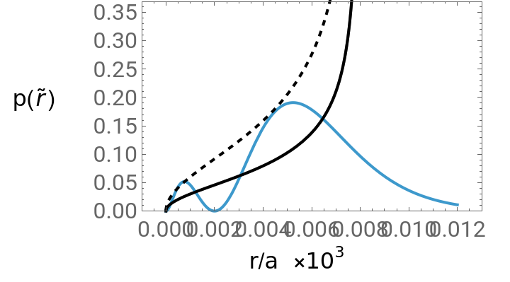
Here, we used the manipulate code. To generate our figure in the paper, we set n=10, n=50 and n=100 as our paper illustrated.
ManipulateShowPlot,{x,0,0.003n^2},,Plot1000xLaguerreL[n-1,1,2000x/n]^2,{x,0,0.003n^2},Plot,{x,0,0.003n^2},PlotStyle->{Black},Plot,{x,0,0.003n^2},PlotStyle->{Black,Dashed},{n,2,1000}
1
π-
3/2
(n^2)
2
1000x
1
n^2
8(n-1)!
n^3*2*n*n!
-1000x/n
1
π-
3/2
(n^2)
2
1000x
1
n^2
2
π-
3/2
(n^2)
2
1000x
1
n^2


Section1.2: Figure 5
Section1.2: Figure 5
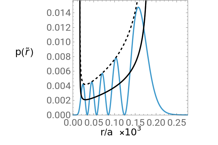
Here, we also used the manipulate code. We set n=10,l=5; n=50,l=25 and n=100,l=50 to generate the figure.
ManipulateShowPlot,x,0.001n^21-,Plot1000xLaguerreL[n-l-1,2*l+1,2000x/n]^2,x,0,0.0015n^21+,x,0.001n^21-,x,0.001n^21-
1+
l^2(l+1)^2
(1000x)^21--1-^2
l(l+1)
n^2
l(l+1)
1000x
π
2n^6-
1
1000x
1
2n^2
1-
,0.0015n^21+l(l+1)
n^2
1-
,l(l+1)
n^2
8*(n-l-1)!
n^3*2*n*(n+l)!
-1000x/n
l
(2000x/n)
1-
,Plotl(l+1)
n^2
1+
l^2(l+1)^2
(1000x)^21--1-^2
l(l+1)
n^2
l(l+1)
1000x
π
2n^6-
1
1000x
1
2n^2
1-
,0.001n^21+l(l+1)
n^2
1-
,PlotStyle->{Black},Plotl(l+1)
n^2
2
1+
l^2(l+1)^2
(1000x)^21--1-^2
l(l+1)
n^2
l(l+1)
1000x
π
2n^6-
1
1000x
1
2n^2
1-
,0.0015n^21+l(l+1)
n^2
1-
,PlotStyle->{Black,Dashed},{n,3,1000},{l,2,n-1}l(l+1)
n^2
Out[]=
Section1.3: Figure 6
Section1.3: Figure 6
Here, we used the manipulate code again. To generate our figure in the paper, we set n=10, l=5,m=1; n=100, l=50,m=10 and n=200, l=100, m=20.
ManipulateShowPlotSqrtCos[xπ]^2+^2×^22πn^3-+SqrtCos[xπ]^2+^2×^22πn^3-,{x,0,1},,Plot(LegendreP[l,m,Cos[xπ]])^2,{x,0,1},PlotSqrtCos[xπ]^2+^2×^22πn^3-+SqrtCos[xπ]^2+^2×^22πn^3-,{x,0,1},PlotStyle->{Black},{n,2,1000},{l,1,n-1},{m,1,l}
l(l+1)
1-
l(l+1)
n^2
1-
1-m^2
l(l+1)
1-
l(l+1)
n^2
1-
m^2
l(l+1)
l(l+1)
1-Cos[xπ]
1-
l(l+1)
n^2
1-
m^2
l(l+1)
1
1--Cos[xπ]*Cos[xπ]
m^2
l(l+1)
21-Cos[xπ]
1-
l(l+1)
n^2
1-
m^2
l(l+1)
l(l+1)
1
n^2
l(l+1)
1-
l(l+1)
n^2
1-
1+m^2
l(l+1)
1-
l(l+1)
n^2
1-
m^2
l(l+1)
l(l+1)
1+Cos[xπ]
1-
l(l+1)
n^2
1-
m^2
l(l+1)
1
1--Cos[xπ]*Cos[xπ]
m^2
l(l+1)
21+Cos[xπ]
1-
l(l+1)
n^2
1-
m^2
l(l+1)
l(l+1)
1
n^2
2l+1
2
(l-m)!
(l+m)!
l(l+1)
1-
l(l+1)
n^2
1-
1-m^2
l(l+1)
1-
l(l+1)
n^2
1-
m^2
l(l+1)
l(l+1)
1-Cos[xπ]
1-
l(l+1)
n^2
1-
m^2
l(l+1)
1
1--Cos[xπ]*Cos[xπ]
m^2
l(l+1)
21-Cos[xπ]
1-
l(l+1)
n^2
1-
m^2
l(l+1)
l(l+1)
1
n^2
l(l+1)
1-
l(l+1)
n^2
1-
1+m^2
l(l+1)
1-
l(l+1)
n^2
1-
m^2
l(l+1)
l(l+1)
1+Cos[xπ]
1-
l(l+1)
n^2
1-
m^2
l(l+1)
1
1--Cos[xπ]*Cos[xπ]
m^2
l(l+1)
21+Cos[xπ]
1-
l(l+1)
n^2
1-
m^2
l(l+1)
l(l+1)
1
n^2
Section1.4: Figure 1
Section1.4: Figure 1
In this figure, we compare the quantum and classical probability density of a harmonic oscillator.
Section2 : (Figure 7)
Section2 : (Figure 7)
The codes below shows how we generate figure 7, which shows the radial eigenfunction of hydrogen model of l=1 and l=0 at different n.
Section3 : (Figure 2)
Section3 : (Figure 2)
The codes below show how we generate the visualization of classical and quantum hydrogen model. In the figure we used in the paper, we adjusted the direction of the 3D figure to make the detail clearer.
CITE THIS NOTEBOOK
CITE THIS NOTEBOOK
How are quantum eigenfunctions of Hydrogen atom related to its classical elliptic orbits?
by Yixuan Yin, Tiantian Wang & Biao Wu
Wolfram Community, STAFF PICKS, December 13, 2024
https://community.wolfram.com/groups/-/m/t/3338816
by Yixuan Yin, Tiantian Wang & Biao Wu
Wolfram Community, STAFF PICKS, December 13, 2024
https://community.wolfram.com/groups/-/m/t/3338816