The Anti-Hawking Effect
is not manifest for a thermal state on massless hyperbolic black holes of three or four dimensions.
Lissa de Souza Campos
University of Pavia - Italy
For criticism, suggestions or requests, please contact me via lissa.campos@alumni.usp.br
is not manifest for a thermal state on massless hyperbolic black holes of three or four dimensions.
Lissa de Souza Campos
University of Pavia - Italy
For criticism, suggestions or requests, please contact me via lissa.campos@alumni.usp.br
Black holes radiate; Hawking radiation is the thermal radiation emitted by a black hole. One way of formalizing this---Hawking effect---is using the concept of a particle detector. A two-level system is a good, simple model of a particle detector, called an Unruh-DeWitt detector. (Imagine an electron of a Hydrogen atom that can be excited or de-excited.) If we put a theoretical particle detector interacting with a quantum state Ψ of a free scalar quantum field theory on a black hole spacetime, we can compute its probabilities of excitation and de-excitation. Probabilities, in turn, can give us thermality. If the transition probabilities of a system behave like an ideal gas in thermal equilibrium, which is Boltzmann Statistics, it yields a temperature, it can be called thermal. When Ψ is a KMS state, aka thermal state, we do obtain a Boltzmann factor for the detector. And this is the Hawking effect: an Unruh-DeWitt detector with energy gap Ω, following static trajectories on Schwarzschild spacetime and interacting with the Hartle-Hawking state, responds such that the ratio between the transition rates of de-excitation per excitation is
ℱ
de-exc.
ℱ
exc.
Ω/
T
H
(
1
)We say the detector thermalized at the Hawking temperature ; the detector measured Hawking radiation.
T
H
The anti-Hawking effect does not work against the Hawking effect; it does not opposes the Hawking effect. It is a negative differential effect, with a somewhat misleading name. It is not an effect that a detector would measure, but it occurs when we compare the response of different detectors in different positions. Usually, the closest to the black hole horizon, the higher the Hawking temperature measured, and there is a one to one correspondence between the fixed spatial coordinates and . The anti-Hawking effect is manifest when the transition rate of the detector, seen as a function only of the Hawking temperature, decreases when increases, hence, a negative differential effect:
T
H
T
H
∂
ℱ
∂
T
H
(
2
)Classically, we could think of the anti-Hawking effect as: “if the temperature is higher, there is more energy around, more collisions, a particle detector should click more, the transition rate should increase.” In this sense, it is a counter-intuitive effect. However, if we are talking about quantum field theory, we can base our intuition with what happens in Minkowski spacetime. From Jorma’s and Lee’s paper, the transition rate of an Unruh-DeWitt detector following Rindler trajectories and coupled to the ground state of a massless scalar field on the four-dimensional Minkowski spacetime is given by:
In[]:=
TransitionMink[4,Egap_,a_]=-1;PlotTransitionMink[4,1/10,a],{a,1/100,5},PlotRangeFull,PlotLabel"Excitation Transition Rate, Ω>0",AxesLabel"a","",PlotTransitionMink[4,-1/10,a],{a,1/100,5},PlotRangeFull,PlotLabel"De-excitation Transition Rate, Ω<0",AxesLabel"a",""
1
2π
Egap
2πEgap
a
ℱ
Mink
4
ℱ
Mink
4
Out[]=
,
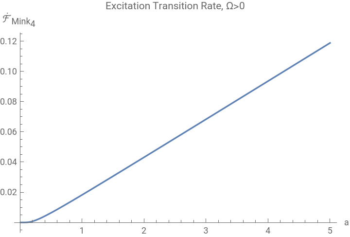
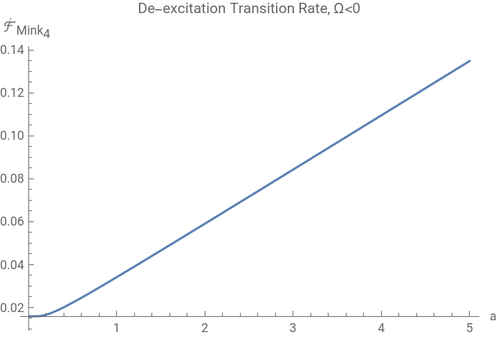
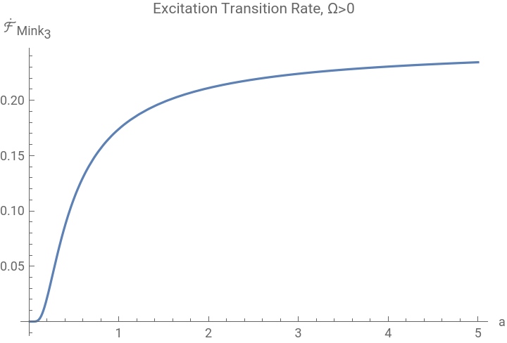
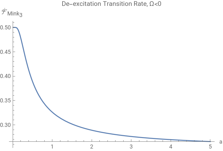
The proper acceleration of each Rindler trajectory is proportional to the local Unruh temperature measured. That is, for both excitations and de-excitations, the transition rate is an increasing function with respect to the local temperature measured by the detector. Based solely on the above, the negative differential effect (2) also seems counter-intuitive---since it does not happen in the four-dimensional Minkowski. However, on the three-dimensional Minkowski spacetime, we have that for de-excitations, the transition rate does decrease with the local temperature:
a
In[]:=
TransitionMink[3,Egap_,a_]=+1;PlotTransitionMink[3,1/10,a],{a,1/100,5},PlotRangeFull,PlotLabel"Excitation Transition Rate, Ω>0",AxesLabel"a","",PlotTransitionMink[3,-1/10,a],{a,1/100,5},PlotRangeFull,PlotLabel"De-excitation Transition Rate, Ω<0",AxesLabel"a",""
1
2
1
2πEgap
a
ℱ
Mink
3
ℱ
Mink
3
Out[]=
,
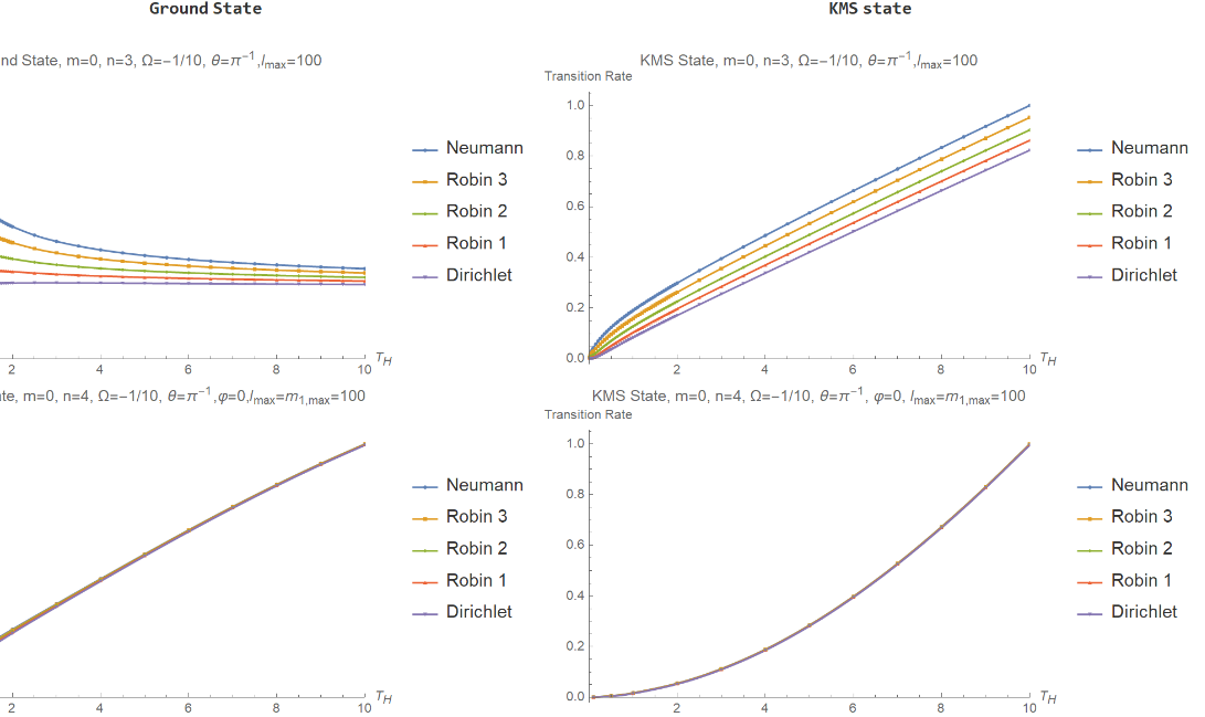
In this notebook, we study the transition rate of an Unruh-DeWitt detector coupled to a ground and to a thermal state of a free scalar massless conformally-coupled quantum field theory on massless hyperbolic black holes of three and four dimensions. We show that it is not manifest for the thermal states in both dimensions and that it is manifest for the ground-state only in three dimensions; summarized in one picture-matrix, we show that:
(
3
)
The results match the behavior in Minkowski. But why is it manifest at all? What does it mean? Why is it manifest in three but not four dimensions? Why is it manifest for the ground state but not for the thermal state? Does it happen in classical physics as well? Maybe in quantum mechanics? Statistics have meaning; I think there is something here to be understood.
If we model the interaction between an Unruh-DeWitt detector, with an energy gap Ω, and a quantum state Ψ by a monopole-type Hamiltonian operator, if we assume the detector is following a static trajectory γ parametrized by its proper time τ, and if the interaction is "turned on" for an infinite proper time interval, then, within first-order of perturbation theory, the instantaneous transition rates of excitation (Ω>0) or de-excitation (Ω<0) are given by the Fourier transform of the two-point function's pullback along the detector's trajectory 〉 and evaluated at the Fourier frequency Ω. That is, to obtain an explicit expression for the transition rate, we need the two-point function; to construct the two-point function, we need to solve the Klein-Gordon equation. This computation is done in detail in our paper “Ground and thermal states for the Klein-Gordon field on a massless hyperbolic black hole with applications to the anti-Hawking effect”. Here, we include the numerical analysis to obtain the results, and part of the computations that are nicely done in Mathematica: checking that the line-elements are solutions of Einstein’s field equations; showing that the Klein-Gordon equation reduces to a hypergeometric equation; and checking the poles of the radial Green function.
(τ)
2
Ψ
Contents
Contents
■ Chapter 0: “Definitions (initialization cells)”: contains the definitions and documentation of all the functions and symbols used in this notebook. The main function is called SetFunctions, with which one can re-set the values of the position of the horizon and the AdS radius. For more information, run all initialization cells and use Help[SetFunctions] or Options[SetFunctions].
■ Chapter 1: “The spacetimes”: contains the line-element of massless hyperbolic black holes and, using the package , shows that it’s a solution of Einstein’s field equations for certain values of cosmological constant and horizon.
■ Chapter 2: “The radial equation”: shows that the radial equation (the equation we are left with after separation of variables on the Klein-Gordon equation) can be written as a hypergeometric equation. This chapter uses the packages: and .
■ Chapter 3: “The poles of the Green function”: illustrates the behavior of the Green function with respect to the frequency ω in the complex plane for different boundary conditions.
■ Chapter 4: “The transition rate on Massless Hyperbolic Black Holes”: this is the main chapter. It contains the numerical analysis to get the plots of the transition rate of the Unruh-DeWitt detector on massless hyperbolic black holes of three and four dimensions. Some computations take time, and for that some data were save in external .txt files.
0. Definitions (initialization cells)
0. Definitions (initialization cells)
1. The spacetimes
1. The spacetimes
Massless hyperbolic black holes are static -dimensional black hole spacetimes with negative sectional curvature which are solutions of Einstein’s field equation in vacuum ), with a negative cosmological constant (Λ):
n
(=0
T
μν
G
μν
Λg
μν
(
4
)Their line element, in Schwarzschild-like coordinates, are given by:
φ
1
φ
n-3
(
5
)L is called the “AdS radius”, the horizon is located at and Σ is an (n-2)-dimensional hyperbolic space. In three dimensions, the hypersurface Σ is just the real line and can be fixed to any positive real number. In four dimensions, Σ is the 2-dimensional hyperbolic space and =L.
r=
r
h
r
h
r
h
Using the package , we can easily study the line-element above. In the following I paste the code of the package---written by Pekka Janhunen---with one minor modification: I removed the symbol CurvatureScalar from the list of blocked symbols.
In[]:=
EinsteinTensor[metric_,x_]:= Block[ {Dim,Metric, PreChristoffel, Christoffel, Riemann, PreRiemann, Ricci,sigma, mu, nu, alpha, beta, gamma}, Dim = Length[x]; Metric = Simplify[Inverse[metric]]; (* Metric with upper indices *) PreChristoffel = Table[ D[metric[[gamma,alpha]],x[[beta]]] + D[metric[[beta,gamma]],x[[alpha]]] - D[metric[[alpha,beta]],x[[gamma]]], {gamma,Dim}, {alpha,Dim}, {beta,Dim} ]; (* The "lower index part" of Christoffel symbols *) PreChristoffel = Simplify[PreChristoffel]; Christoffel = (1/2) Metric . PreChristoffel; (* The full Christoffel symbols *) Christoffel = Simplify[Christoffel]; PreRiemann = Table[ D[Christoffel[[sigma,alpha,nu]],x[[mu]]] + Sum[Christoffel[[gamma,alpha,nu]] Christoffel[[sigma,gamma,mu]], {gamma,Dim} ], {sigma,Dim}, {alpha,Dim}, {mu,Dim}, {nu,Dim} ]; (* PreRiemann has to be antisymmetrized to yield Riemann tensor: *) Riemann = Table[ PreRiemann[[sigma,alpha,mu,nu]] - PreRiemann[[sigma,alpha,nu,mu]], {sigma,Dim}, {alpha,Dim}, {mu,Dim}, {nu,Dim} ]; Ricci = Table[ Sum[Riemann[[sigma,alpha,sigma,beta]], {sigma,Dim}], {alpha,Dim}, {beta,Dim} ]; CurvatureScalar = Sum[ Metric[[alpha,beta]] Ricci[[alpha,beta]], {alpha,Dim}, {beta,Dim} ]; (* Return Einstein tensor: *) Ricci - (1/2) CurvatureScalar metric ]
Three dimensional case:
Three dimensional case:
And its scalar curvature is:
Four dimensional case:
Four dimensional case:
Then the cosmological constant is:
And its scalar curvature is:
2. The Klein-Gordon equation
With the ansatz
Let λ be the eigenvalue of Y. Both equations above reduce to the following O.D.E, called the radial equation:
First, we show that it can be reduced to a hypergeometric equation. Then, we obtain the measure with respect to which the solutions must be square-integrable.
As a hypergeometric equation
As a hypergeometric equation
First, applying the transformation on the independent variable:
we get:
Asymptotically, we have:
Defining the auxiliary parameters:
And considering the ansatz:
we obtain that (9) solves the radial equation if and only if h[z] solve the hypergeometric equation
with coefficients given by:
Now we must solve a system to determine a and b:
With the auxiliary definitions:
we write the parameters of the Hypergeometric equation as:
Equivalently, using the definition of β:
In Sturm-Liouville form
In Sturm-Liouville form
The equation in Sturm-Liouville form is given by:
The measure w.r.t. the solutions must be square-integrable is given by:
The weight function that appears in the normalization of the radial Green function is given by:
And the potential:
3. The poles of the Green function
3. The poles of the Green function
In chapter 0, we defined the functions Ξ and the function H:
The argument principle states that the number of zeros Z and poles P of f satisfy:
Knowing P, and studying this integral, we can obtain Z.
Three Dimensional case:
Three Dimensional case:
Consider the parameter set:
For these values, and assuming Im[ω]<0, the function H has one zero and no poles. We can see this by:
1) Checking that
The integral over the real line seems to be converging to 1:
The arc integral is close to zero:
The argument above is not a proof; but corroborates our claim.
For purely imaginary frequencies, the function Ξ is real valued. In this case. And for negative Im[ω], it is bijective:
2) Using ComplexPlot3D, we can see the zeros and poles of H in a certain region of the complex plane:
On the other hand, for
there are no zeros:
Four Dimensional case:
Four Dimensional case:
For certain boundary conditions, H has one zero:
For others, no zero:
4. The transition rate on massless hyperbolic black holes
4. The transition rate on massless hyperbolic black holes
Chapter 0 contains the definitions of the transition rates of an Unruh-DeWitt detector coupled to a ground and a KMS state of a massless conformally-coupled scalar field on three and four dimensional massless hyperbolic black holes.
The transition rates are products of very small numbers by very large numbers---so we need to check the precision settings carefully; and for each parameter set.
The transition rates are products of very small numbers by very large numbers---so we need to check the precision settings carefully; and for each parameter set.
Three dimensional case:
Three dimensional case:
For n=3, I have defined the functions
For the KMS state, analogously:
To understand the global behavior, is better to check the transition rate with respect to z, using the first function. But to see the anti-Hawking effect, is better w.r.t the local Hawking temperature T, using the second function.
Transition rate for the ground state of a massless field as a function of temperature, Ω = - 0.1
Transition rate for the ground state of a massless field as a function of temperature, Ω = - 0.1
Transition rate for the KMS state of a massless field as a function of temperature, |Ω| = 0.1
Transition rate for the KMS state of a massless field as a function of temperature, |Ω| = 0.1
Four dimensional case:
Four dimensional case:
For n=4, I have defined the functions
For the KMS state, analogously:
Transition rate for the ground state of a massless field as a function of temperature, Ω = - 0.1
Transition rate for the ground state of a massless field as a function of temperature, Ω = - 0.1
Transition rate for the KMS state of a massless field as a function of temperature, |Ω| = 0.1
Transition rate for the KMS state of a massless field as a function of temperature, |Ω| = 0.1
References
References
In this notebook, we reproduce the results of the paper “Ground and thermal states for the Klein-Gordon field on a massless hyperbolic black hole with applications to the anti-Hawking effect”, doi: 10.1103/PhysRevD.103.025021
which was inspired by
The BTZ black hole exhibits anti-Hawking phenomena. doi:10.1016/j.physletb.2020.135732
which was inspired by
The BTZ black hole exhibits anti-Hawking phenomena. doi:10.1016/j.physletb.2020.135732