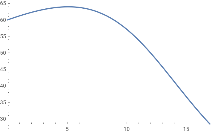
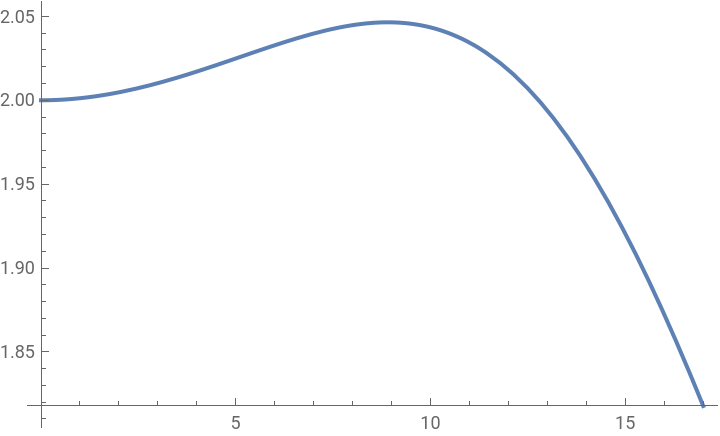
WolfPopulationDynamics::usage="The following differential equations represent the pattern of interaction between deer, coyotes and wolves in Yellowstone. The initial amounts are in thousands. It is observed that the increase in the coyote population increases competition and then causes a decrease. But the interaction between coyotes and deer has a positive impact, because there is more food. The equations are: E1'[t] = 0.04E1[t]-0.003E1[t]C1[t]-0.85E1[t]W1[t] C1'[t] = -0.06C1[t]+0.001E1[t]C1[t] W1'[t] = -0.12W1[t]+0.005E1[t]W1[t] References: Zill, D.G. and Cullen, M.R. Differential Equations with Boundary-Value Problems. Ed. Brooks/Cole: pp.69-71, 1997.; Personal.";
In[]:=
diffeqs[{E10_,C10_,W10_}]:={E1'[t]==0.04E1[t]-0.003E1[t]C1[t]-0.85E1[t]W1[t],C1'[t]==-0.06C1[t]+0.001E1[t]C1[t],W1'[t]==-0.12W1[t]+0.005E1[t]W1[t],E1[0]==E10,C1[0]==C10,W1[0]==W10};endTime=17;initPt={60,2,0.015};soln=Flatten[NDSolve[diffeqs[initPt],{E1,C1,W1},{t,0,endTime}]]
Out[]=
E1InterpolatingFunction,C1InterpolatingFunction,W1InterpolatingFunction


In[]:=
Plot[Evaluate[E1[t]/.soln],{t,0,17},PlotRangeAll]
Out[]=
In[]:=
Plot[Evaluate[C1[t]/.soln],{t,0,17},PlotRangeAll]
Out[]=
In[]:=
Plot[Evaluate[W1[t]/.soln],{t,0,17},PlotRangeAll]
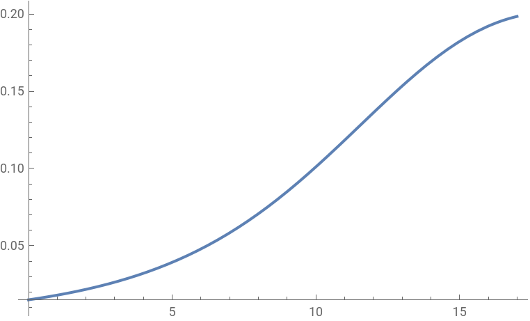
It is observed that the only growing population, successfully, that of wolves, despite their small initial number. Wolves act with strategy.