For my summer school project, I decided to program a classic microeconomics problem that was first brought to life in the seminal paper written by K. Sridhar Moorthy (1984). This paper sheds light on the topic of market segmentation under third-degree price discrimination, where customers cannot be targeted by personalized prices or products and instead get to self-select from a list of price-quality menu. In my project, I modelled this one-shot sequential game between a single firm (i.e., monopoly) and a population of customers with heterogeneous intensity of preference for quality (an example attribute of a product). I extend Moorthy’s model by allowing for customers to be heterogeneous in their budgets as well. My code provides flexibility to try different parameters and functions as inputs of this game. Examples of customer-related inputs are 1)willingness-to-pay function (usually an increasing function in quality), 2)distribution of “customers’ intensity of preference for quality” and 3)distribution of “customers’ budget levels”. Examples of firm-related inputs are 1)number of products (m), 2)cost function and 3)potentially capacity constraints. Such flexibility is very useful for researchers in this field to numerically investigate different scenarios and build up strong intuition about the optimal results.
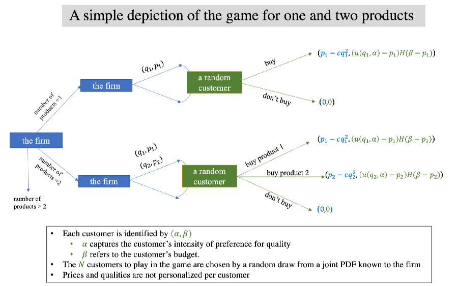
The sequence of events in this game are as follow:
◼
The firm chooses how many products to offer
◼
The firm then selects a price-quality menu for their product line
◼
The customers self-select which product to buy.
Out[]=
Next, I explain the main steps of the code:
Section 1: Defining the game inputs
Section 1: Defining the game inputs
In this section, we will define the inputs of the problem for both players.
1-1: Inputs related to player 1: Customers
1-1: Inputs related to player 1: Customers
Every customer in the market is identified by a pair of parameters (α , β):
◼
α ∈ [αmin,αmax] captures a customer’s intensity of preference for quality
◼
β ∈ [βmin, βmax] captures a customer’s budget to spend on this firm’s products.
In[]:=
αmin=0;αmax=1;βmin=0;βmax=4;
Next, let us define a PDF for both variables α and β. In this version of the code, these two variables are assumed to be independently distributed. However, it is plausible to define a dependent joint distribution as well.
In[]:=
αDistribution=TriangularDistribution[{αmin,αmax}];βDistribution=TriangularDistribution[{βmin,βmax}];jointcustomerDistribution=ProductDistribution[αDistribution,βDistribution];
From the jointcustomerDistribution, we randomly draw 100 customers to play in this game :
In[]:=
customercounter=100;customerPopulationlist=RandomVariate[jointcustomerDistribution,customercounter];
Here, we see the customer distribution (on the left) and the histogram sample of customers that enter the game (on the right)
In[]:=
Grid[{{Panel[Labeled[Plot3D[PDF[jointcustomerDistribution,{α,β}],{α,αmin,αmax},{β,βmin,βmax},AxesLabel{Style["α",FontSize15,Bold,Red],Style["β",FontSize15,Bold,Red]},ImageSize300],Style["Joint PDF of α and β",FontFamily"Garamond",FontSize15],Top]],Panel[Labeled[Histogram3D[customerPopulationlist,10,"ProbabilityDensity",AxesLabel{Style["α",FontSize15,Bold,Red],Style["β",FontSize15,Bold,Red]},ImageSize300],Style["Random Sample Size of "<>ToString[customercounter]<>" Drawn from Customer Distribution",FontFamily"Garamond",FontSize15],Top]]}}]
Out[]=


◼
customerutility[] is an increasing function in α and quality. This function captures the customer’s willingness -to-pay for a product of quality level q.
◼
surplusFunction[] reads quality and price of a particular product and simply returns the net utility (i.e., utility - price) if the customer can afford to buy the product and 0 otherwise.
In[]:=
customerutility[q_,α_]:=αq;surplusFunction[α_,β_,q_,p_]:=Boole[p≤β](customerutility[q,α]-p);
1-2: Inputs related to player 2: Firm
1-2: Inputs related to player 2: Firm
Next, we define the parameters of the game for the firm.
It is a common assumption that unitCost[] is convex increasing in quality.
It is a common assumption that unitCost[] is convex increasing in quality.
In[]:=
numberofproducts=3;costparameter=0.1;unitCost[q_]:=costparameter;
2
q
Section 2 : Main functions of the game
Section 2 : Main functions of the game
We next need to construct the market demand function. I approach this task by first solving the surplus maximization problem for every customer in our sample population and then counting all the customers who self-select each product.
In[]:=
customerSurplusFunction[α_,β_,qlist_,plist_]:=Map[surplusFunction[α,β,#〚2〛,#〚1〛]&,Thread[{plist,qlist}]]customerDemandFunction[α_,β_,qlist_,plist_]:=If[Max[#]>0,First@Ordering[#,-1],0]&@customerSurplusFunction[α,β,qlist,plist]marketDemandFunction[j_,qlist_,plist_]:=Count[customerDemandFunction[#〚1〛,#〚2〛,qlist,plist]&/@customerPopulationlist,j]profitFunction[qlist_,plist_]:=Total[marketDemandFunction[#,qlist,plist](plist〚#〛-unitCost[qlist〚#〛])&/@Range@numberofproducts]
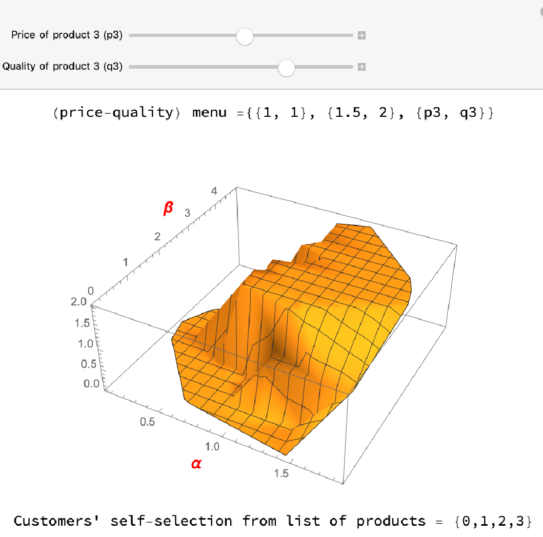
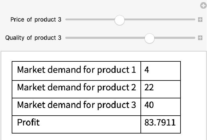
Here is an example of customers’ demand function for a given price-quality menu. The height of the following 3D plot indicates the index of self-selected product. It is easy to see that the demand for product 3 increases in its quality or decreases in its price and the profit seems to have an interior maximizer.
Section 3 : Running the game (the optimization)
Section 3 : Running the game (the optimization)
3-1: Creating the search space
3-1: Creating the search space
Our optimization approach is simply discretizing the continuous space and search over all the discrete points for the best solution.
◼
The following (first) set of formulas aim to construct us a search space for our upcoming optimization problem.
◼
qstep and pstep refer to steps to divide the quality continuum and price continuum.
◼
mainSearchSpace is a list containing all the price-quality menu choices for the firm to investigate (it is the game field for the firm)
◼
qmax refers to maximum quality level that the firm can strive for.
3-2: Finding the profit maximizers
3-2: Finding the profit maximizers
◼
This is the main part of the model where the profit function is being optimized over the discretized space.
◼
In profitlist, we calculate the profit all the points in our mainSearchSpace (not quite efficient!)
◼
optimalProfit[] simply returns the maximum of profitlist.
◼
setofAllOptimalsolutions returns all the points in the mainSearchSpace that have achieved the maximum profit.
◼
Depending on the fineness of mainSearchSpace and the shape of the customerPopulationlist and its size, we might locate a unique maximizer or multiple maximizers. For example:
◼
in a search space with qstep=1 and pstep=1 (that contains 144 points), we locate five maximizers that achieve the profit of 23
◼
in a search space with qstep=1 and pstep=0.5 (that contains 759 points), we locate 1 maximizer that achieve the profit of $31.5
◼
in a search space with qstep=0.5 and pstep=0.5 (that contains 7732 points), we locate 4 maximizers that achieve the profit of $32.5
◼
The smaller the steps, the closer the solution will be to true optimal. There is an inherent trade-off between the granularity of search space (i.e., accuracy of search) and optimization processing time.
Future Extensions
Future Extensions
◼
The current code searches over a discrete space. There is a natural trade-off between the granularity of the search space and the processing time.
◼
Running the optimization for different combination of “Model Inputs”, store the results and run sensitivity analysis of optimal results relative to critical parameters of the model (e.g., three products vs. two products)
◼
Next steps: Enriching the problem by:
◼
Allowing for non-unitary demand (some customers might want to buy multiple products)
◼
Incorporating constraints such as capacity constraints for the firm’s profit optimization
◼
Incorporating a second firm and capturing competition (duopoly)
◼
Running a “dynamic” pricing model where the state of the world updates at the beginning of every discrete-time period. Examples of the state of the world may include “customer distribution”, “customers’ purchase history” or “financial profile of the firm”
Keywords
Keywords
◼
Optimization
◼
Pricing
◼
Market segmentation
◼
One-shot sequential game
◼
Product line decisions
Acknowledgment
Acknowledgment
Mentor: Ahmed Elbanna
Special Thanks go to my mentor Ahmed Elbanna and the awesome team of TAs: Mark Greenberg, Carlos Muñoz and Robert Mendelsohn,
References
References
◼
K. Sridhar Moorthy, 1984. “Market Segmentation, Self-Selection, and Product Line Design,” Marketing Science, INFORMS, vol. 3(4), pages 288-307.