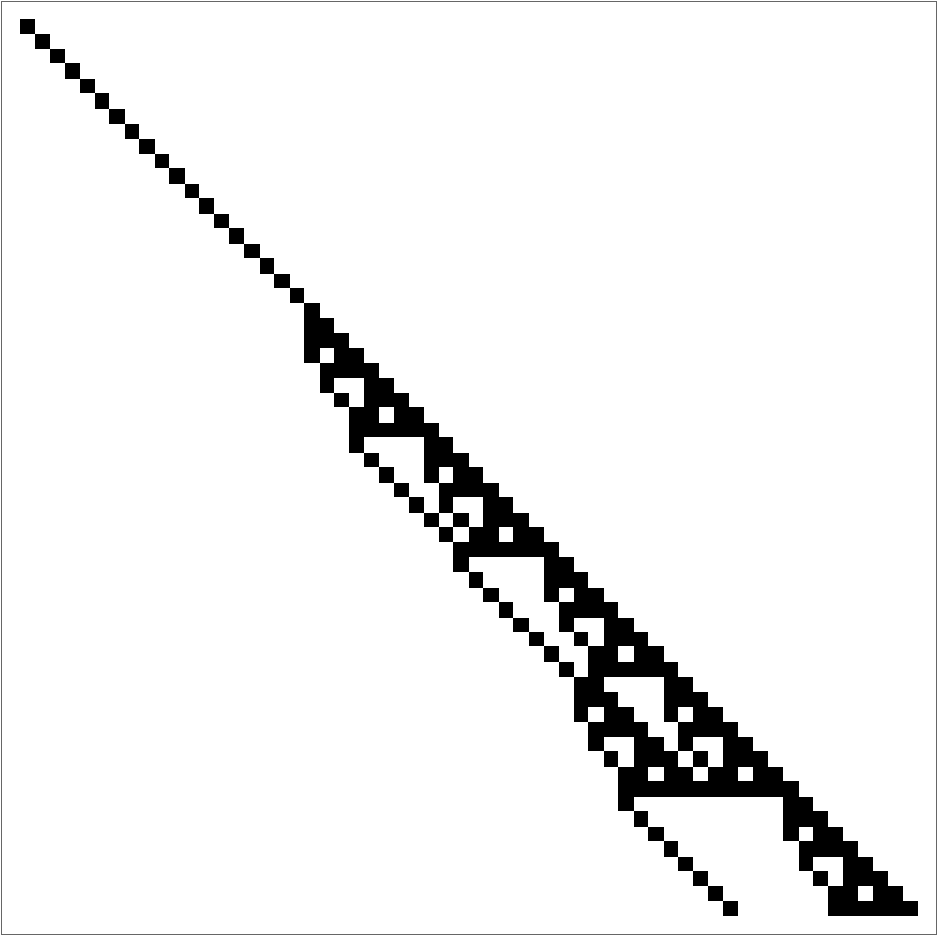
The goal of this project is to classify and investigate particle like structures in cellular automata (CA). I will first create the particles using different CA rules, and study their motion by examining the patterns of their trails. I will then evaluate their behavior by changing the initial conditions and introducing perturbations, which emulate external forces or obstacles that alter the state of the system.
Introduction
Introduction
This project is an attempt at a phenomenological analysis with the goal of analyzing and categorizing particle-like structures in CA. Such computational systems can generate complex patterns from simple initial conditions and interactions that evolve over time. For the purposes of this project, a “particle” is defined as a localized structure that travels over the CA space over time and leaves a discernible trace.
I will start by creating and classifying particles using different CA rules. This involves analyzing the different patterns of the trails to determine how they travel. Afterwards, I will survey their behavior under different settings by changing the initial conditions and adding perturbations to their tracks. These perturbations act as outside forces or physical barriers that alter the system’s condition at a specific time and evolution step. The main goal will be to watch how particles react to external stimuli and interpret the resulting behaviors.
I will start by creating and classifying particles using different CA rules. This involves analyzing the different patterns of the trails to determine how they travel. Afterwards, I will survey their behavior under different settings by changing the initial conditions and adding perturbations to their tracks. These perturbations act as outside forces or physical barriers that alter the system’s condition at a specific time and evolution step. The main goal will be to watch how particles react to external stimuli and interpret the resulting behaviors.
Definition of a “particle”
Definition of a “particle”
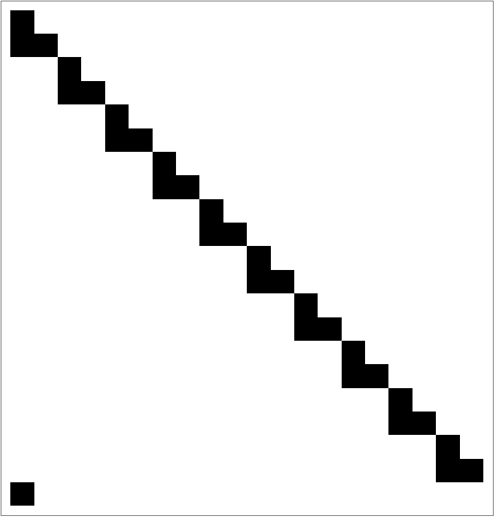
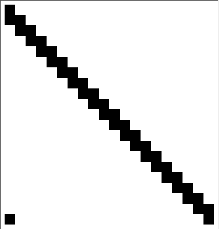
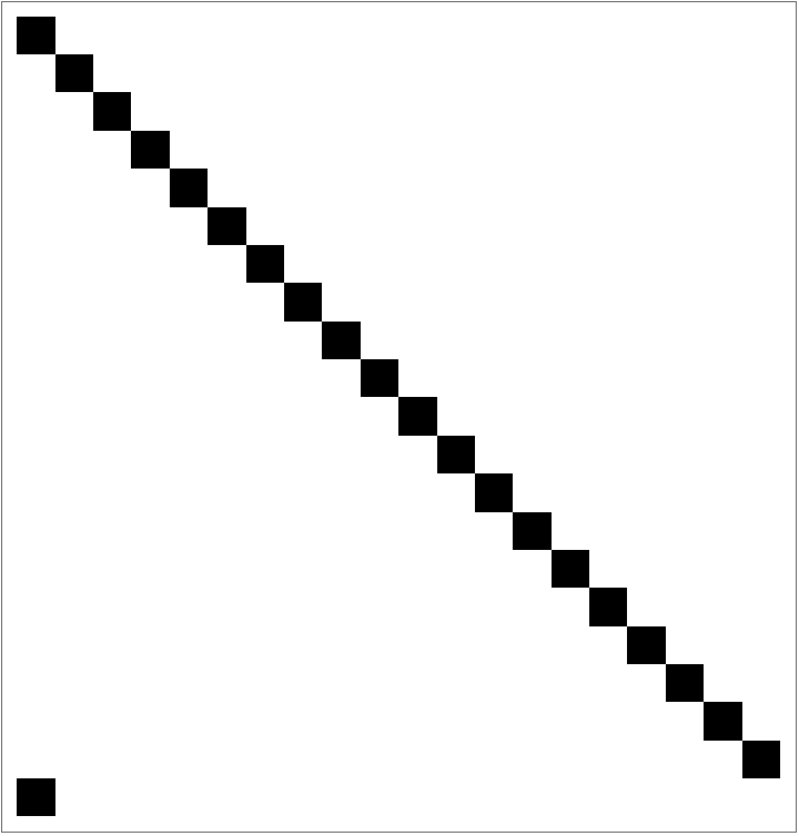
Physically, particles can be defined as objects whose properties remain unchanged throughout space and time. With that in mind I defined a particle in the context of CA as a localized, persistent structure that moves through the CA lattice, preserving its identity over time and interacting with other particles or structures. These particles can be visually represented by trails, which are distinct, periodic patterns of cells that emerge, maintain coherence, and propagate through the grid. The trails indicate the particle’s trajectory and behavior, with time flowing downwards. I identified three patterns that they follow:
Type A:
Out[]=
Type B:
Out[]=
Type C:
Out[]=
It is important to mention that each pattern can be generated by multiple rules, and each generate different results when a perturbation is introduced. For the sake of brevity, I will only focus on some specific rules that I considered to have the most interesting results. These rules are:
◼
20 for A
◼
120, 184, and 240 for B
◼
212 and 244 for C
Meaning of the patterns
Meaning of the patterns
The differences of the shapes and patterns of each trail can shed light on the motion of the particle:
◼
Type C indicates that the particle travels to the next cells at a constant speed, given that the black cells are diagonal to each other.
◼
The vertical segments of the trails of type A represent the particle remaining stationary on the same cell. Then, it quickly moves to the next cell at the exact time when the stationary behavior ends, indicated by the horizontal lines. Finally, it moves to the following cell with constant velocity, exhibiting the same diagonal pattern as C until the cycle repeats.
◼
Type B shows the same vertical lines and horizontal lines as type A, but there are no diagonal blocks. This means the particle has a more erratic motion pattern, alternating between rests and quick transitions to the next cells.
Perturbations
Perturbations
To better categorize their behaviors, I perturbed the initial conditions and observed the results. The following code applies a perturbation on the particle at a specific step. Physically, this perturbation represents an external influence or event that modifies the state of the system at a given point in time. It takes the configuration of the system just before the perturbation step, alters a particular cell to create a “disturbance” (like a new particle or an obstacle), and then continues the evolution of the cellular automaton from this perturbed state. This can model scenarios such as a particle collision, the introduction of a defect, or any other sudden change in the system’s dynamics. The interactive controls of the picture function alter the cell which the perturbation will occur at.
In[]:=
applyPerturbation[rule_, initialcondition_, time_, step_, perturbation_] := Module[{evolution = CellularAutomaton[rule, initialcondition, step - 1]}, Join[evolution, CellularAutomaton[rule, perturbation, time - step]]];picture[rule_, initialcondition_] = Manipulate[applyPerturbation[rule, initialcondition, 60, 20, ReplacePart[Last@CellularAutomaton[rule, initialcondition, 20], {cell -> 1}]] // ArrayPlot, {cell, 1, 60, 1}, SaveDefinitionsTrue];
Below are the initial conditions I used and their physical meanings
◼
Single particle
In[]:=
initialcondition1=ReplacePart[ConstantArray[0,60],1->1];
◼
Beam of particles
In[]:=
beam=ReplacePart[ConstantArray[0,60],(1|3|5)->1];
◼
Beams at random places
In[]:=
SeedRandom[123];randomBeams=RandomInteger[1,60];
I also modified the perturbation so that it represents two particles side by side. I did so by adjusting the picture function:
In[]:=
pictureModif[rule_, initialcondition_] = Manipulate[applyPerturbation[rule, initialcondition, 60, 20, ReplacePart[Last@CellularAutomaton[rule, initialcondition, 20],{cell -> 1, cell+21}]] // ArrayPlot, {cell, 1, 60, 1}, SaveDefinitionsTrue];
Behaviors After Perturbation
Behaviors After Perturbation
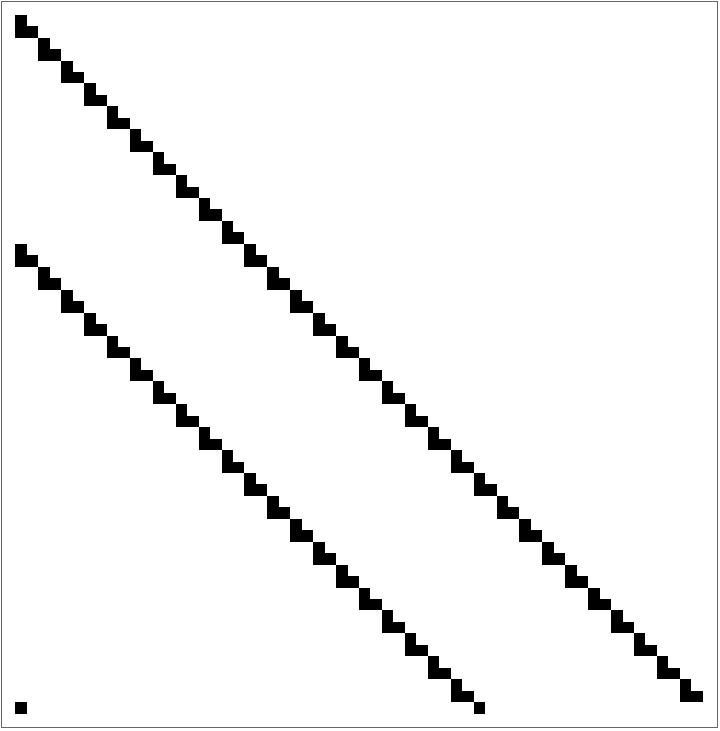
After perturbing those initial conditions, I observed the following behaviors according to each rule. The convention here is that the perturbation (the shorter trail) approaches from left to right.
Rule 20
Rule 20
The incoming perturbation vanishes just when it is two cells to the left of the main trail, suggesting that the perturbation and the main trail interact in such a way that the perturbation is annihilated at that specific location. However, it reappears when it moves to the next cell, and it is linked to the main trail, implying the creation of a new particle at the cell. The perturbation’s disappearance and subsequent reappearance indicate a possible process by which this particle can interact to undergo annihilation and then creation.
Single particle
In[]:=
picture[20,initialcondition1]
Out[]=


Beam of particles
Random beams
Modified perturbation
Rule 120
Rule 120
Strange decay patterns are produced when the perturbation approaches from the left and interacts with the main trail, creating multiple trails. They represent particles moving at various speeds due to the wide range of slopes of the resulting trails, which adds to the complexity of the behavior. This interaction could signify a complex decay process where a massive particle decays into smaller ones when perturbed.
However, the patterns disappear once the perturbation is two or more cells away (right or left) from the main trail. The absence of decays at this range of cells indicates that the interaction only occurs at close proximity with the particle, which is also evident when two or more trails are in contact with each other at the random beams scenario.
However, the patterns disappear once the perturbation is two or more cells away (right or left) from the main trail. The absence of decays at this range of cells indicates that the interaction only occurs at close proximity with the particle, which is also evident when two or more trails are in contact with each other at the random beams scenario.
Single particle
Beam of particles
Random beams
Modified perturbation
Rule 184
Rule 184
The trail splits into two trails when the perturbation approaches to the left of the main trail and when it is about to reach the opposite side to the right. This behavior could be related to a decay into new particles. However, the decay process appears to be much less complex than the one observed with rule 120, indicating that the particles under this rule are probably not very reactive. This simplicity is also evident when the initial conditions involve random beams.
Single particle
Beam of particles
Random beams
Modified perturbation
Rule 212
Rule 212
There seems to be a repulsive force at very specific locations, particularly two cells to the right of the main trail. Beyond this range, the force vanishes and the trails merge together. This force is also observed on multiple trails as in the scenario with the beam of particles, and, interestingly, it does not seem to decrease with distance from the perturbation. Instead, it acts evenly on all of the beams, displacing them by equal distances. Further, when the perturbation is modified to two beams, the range of the repulsive force increases from 2 cells to 4 cells, indicating that the force might be proportional to the number of incoming perturbations.
Single particle
Beam of particles
Random beams
Modified perturbation
Rule 240
Rule 240
The particle seems to not be reactive at all, no matter the perturbation or the initial condition. The perturbation passes through the trails without any dramatic changes. Because of that, they can stay in contact with each other without causing processes such as decays, as evidenced by the darker patches in the random beams scenario
Single particle
Beam of particles
Random beams
Modified perturbation
Concluding Remarks
Concluding Remarks
This project has analyzed and categorized how particle-like structures in CA interact with each other. I have discovered several behaviors by characterizing the particles by CA rules and trails, and applying perturbations to the initial conditions. Some included simple decay and annihilation processes as observed in rules 184 and 20. Others exhibited complex decay patterns such as rule 120, and others showed strange repulsive forces like rule 212.
Possible future developments for this project may involve the use of more complex perturbations and the use of conservation laws of particle physics to better understand the behavior of these particles and relate them to the particles of the Standard Model.
Possible future developments for this project may involve the use of more complex perturbations and the use of conservation laws of particle physics to better understand the behavior of these particles and relate them to the particles of the Standard Model.
Acknowledgments
Acknowledgments
I would like to thank my mentors Gianmarco Morbelli and Jon Lederman for providing the needed guidance to write the code for this project. I am also thankful for the input and advice provided by Xerxes Arsiwalla. Finally, I extend my special thanks to Stephen Wolfram for suggesting me this project.
References
References
1
.A. J. Larkoski (2019), Elementary Particle Physics: An Intuitive Introduction. Cambridge.
2
.F. Berto and J. Tagliabue (2012), “Cellular Automata,” Stanford Encyclopedia of Philosophy. https://plato.stanford.edu/entries/cellular-automata/#toc.
3
.Cite This Notebook
Cite This Notebook