In the Wolfram Model, the underlying geometry of the manifold reflects in many way in the structure of the hypergraphs. In particular, the curvature of a space-like hypersurface clearly reflects in the number of spatial edges of the sprinkled-generated spatial graph representing it. In the General Relativity framework, a Scalar Field (for instance, matter) has a direct effect on this quantity – as evident from the Relativistic Lagrangian – but (mirroring the Equivalence Principle) form the Einstein Field Equations it is impossible to actually recover any information on what exactly depend on the curvature of the spacetime, and what on the Scalar Field. The goal of the project is then twofold: to infer these effects from a given Scalar Field configuration, and (without any previous knowledge of the Manifold) to actually recover information about the presence of the Scalar Field itself.
Introduction
The Einstein Field Equations (EFE) in General Relativity (GR) are proved to be unique by Lovelock’s Theorem. In such configuration, the Gravitational Field is completely described by (up to second derivatives of) the metric tensor, and the Field Equations can be derived by extremizing Hilbert’s Action (in vacuum):
S
GR
-g
R4
(
1
)where is the Ricci Scalar and is the determinant of the metric tensor. The presence of matter only slightly changes the form of the equations, as the Energy-Momentum Tensor of a decoupled Matter Field is yet another functional derivative of the Action. The immediate effect of this approach is that curvature and (the presence of) matter are intrinsically connected, and certainly indistinguishable at the level of the EFE – in virtue of the Strong Equivalence Principle and the Principle of General Covariance.
R
g
Whatever the matter configuration, it is then always possible to reincorporate its effect in the geometry of the manifold, by constructing a particular metric that approximates it with an arbitrary level of precision. Historically, one of the most studied metric transformations are conformal transformations, that transform the metric as:
*
g
μν
2
A
g
μν
(
2
)with the so called conformal factor – the square exponent is a convention to indicate that the choice of the conformal factor does not modify the sign of the metric. While two conformal frames are (far from singularities) mathematically equivalent, they are not at all physically so: this is extremely relevant, as in GR it is preferable to specify the metric and the Energy-Momentum Tensor independently, on the basis of physical consideration, and use conformal frames only when in search of particular effects. It is the case of Alternative Theories of Gravity, formally constructed by weakling (or modifying) some (or all) assumptions of Lovelock’s Theorem. For Scalar-Tensor Theories (STT), the hypothesis that the components of the second-order Einstein Tensor are concomitants of only the metric tensor is dismissed, and (in a conformal frame) a Scalar Field is therefore minimally coupled with the (tensorial) Gravitational Field; in this formulation, the Action is then:
2
A
φ
S
STT
-
*
g
*
R
μν
*
g
φ
,μ
φ
,ν
4
S
M
2
A
Ψ
M
(
3
)where ) highlights the conformal choice. It is evident, from the Lagrangian, that in this conformal frame the Matter Field is then not independent from the Scalar Field. The question of how to distinguish between the pure geometrical aspects and any coupled field is, therefore, extremely relevant.
(*
Scalar Field’s Geometrical Effects
Scalar Field’s Geometrical Effects
In a casual graph, the underlying structure of spacetime translates to the (density of) casual edges, as they are added to a sprinkling in accordance with the metric of the embedding manifold. In general, any information on the geometry should be recovered by the edges, as any vertex does not contain any coordinate label, and this is certainly the case for many proprieties of the casual graph (curvature, dimensions, etc.). On the other hand, when considering a sprinkling directly generated on a manifold of known algebraic curvature, the coordinate information is still conserved in the graph, and the positions of the vertices in relation to each other, as well as the densities of edges, directly correlate with the underlying geometry of the spacetime. The following is an example of a sprinkling of 100 points into a 2+1 dimensional curved spacetime, visualized by taking into consideration the coordinate labels. In a way, each vertex corresponds to an event in the spacetime.
Out[]=

Starting from a vertex, the set of all other vertices that can be reached following casual edges can be seen as representing the light cone of the event. This means that each edge represents a timelike direction between vertices, and those which cannot be reached are spacelike separated. By choosing a particular set of spacelike separated vertices, a spacelike hypersurface is then selected. The resulting graph is called a Spatial Hypergraph, and the following is an example of a sprinkling of 200 points into a 3-dimensional Riemannian manifold with a specified intrinsic curvature function.
Out[]=
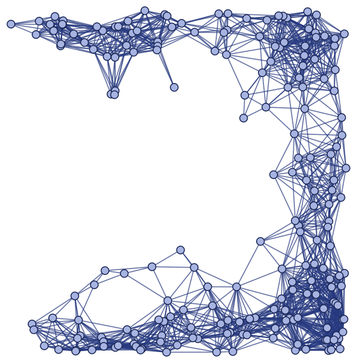
In a spatial (hyper)graph, the density of spatial edges is such that an approximate isometry between the spatial graph and the underlying manifold is guaranteed, as a function of both the discreteness scale and the specified curvature. In light of the previous discussion on the nature of the curvature, it is reasonable to ask if it would be possible to distinguish the pure geometrical effect from the presence of, for instance, a particular matter configuration. While, in general, the answer is clearly no, it is still relevant to ask if some information could be recovered by assuming a background curvature; this is physically consistent, as it is always the case that the metric is assumed in the model, and any other field is additionally specified. The first step would be to recover a specified scalar field configuration, by looking at some difference in the proprieties of spatial graphs: in general, it is not straightforward to imagine that much more than some degree of incompatibility can be actually recovered from such an approach. Surprisingly, it will be shown that (at least in the case in which the coordinate label are preserved) it is indeed possible to reconstruct the Scalar Field, with increasing accuracy as a function of different properties of the spatial graph.
Reconstructing the Scalar Fields
No assumptions are made on the form of the Scalar Field, as every configuration has the same direct effect on the properties of the spatial graph, because the spatial edges only depends on the norm between two points, and the Scalar Field is implemented at that level. In particular, the norm is adjusted, point by point, by the value of the Scalar Field in that point: in this way, where the Scalar Field has a higher value, there will be an higher density of edges in the (surrounding region of the corresponding vertex of the) spatial graph. For simplicity, a Scalar Field in the shape of a binormal distribution is used, centered at and with covariance matrix:
,
1
2
1
2
;
0.4 | 0.04 |
0.04 | 0.4 |
the normalized probability density function is represented in the following picture:
Out[]=

The degree of approximation of the recovered value of the Scalar Field will be given in terms of asymptotics of the mean squares distance from the analytical value, providing a first, rudimentary idea of the correctness of the recovery process. This would depend, in general, on many parameters involved in the discretization of the curved slice (in the following, three parameters are identified: the number of points, the discretization scale, the coupled constant plus an additional curvature factor that will be used to explore similar but increasingly curved spacetime, and that therefore lacks any particular asymptotics, meaning that every curvature can be considered independent from the others). The details of the calculations will be explained in due course.
It is nonetheless known that the norm is not uniform through the whole graph; even less so in the case of different sprinklings of the manifold. It will be necessary to find a way to compensate for this lack of generality (using some local considerations), and this too will be addressed in the following (this is also a reason behind the choice of using personally defined functions to generate the spatial graphs, limiting the use of the functions already present in the Function Repository to the generation of the sprinkling and its graphical representation). In first instance, the simpler case of flat (Minkowski) spacetime would help providing an intuition of the problem without taking into consideration this problematic behaviour, while still resulting in a sufficiently robust implementation that could be easily generalized to curved spacetime configurations.
Flat Manifold
Flat Manifold
In the Function Repository, the function “FlatManifoldToGraph” is already present and well-documented. It allows one to generate a sprinkling into a Minkowski manifold with a given amount of points, and a vertex degree that correlates to a given discreteness scale. This would suffice for this first step, but as the Scalar Field must be implemented at the level of the norm, this function is defined first:
In[]:=
FlatSprinkling[a_,b_]:=Module[{edgeList,dimensions,pointsCount,discretenessScale,points,originalGraphf},edgeList={};dimensions=2;pointsCount=Round[a];discretenessScale=b(1+);points=Take[ResourceFunction["FlatManifoldToGraph"][dimensions,discretenessScale,pointsCount]["PointsList"],pointsCount];Module[{point=#},(If[(Norm[point-#])<discretenessScale,edgeList=Append[edgeList,UndirectedEdge[point,#]]])&/@points]&/@points;{points,edgeList}];
2
10
-1
10
-dimensions
a
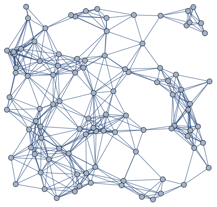
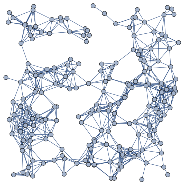
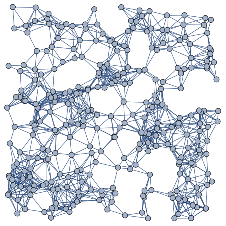
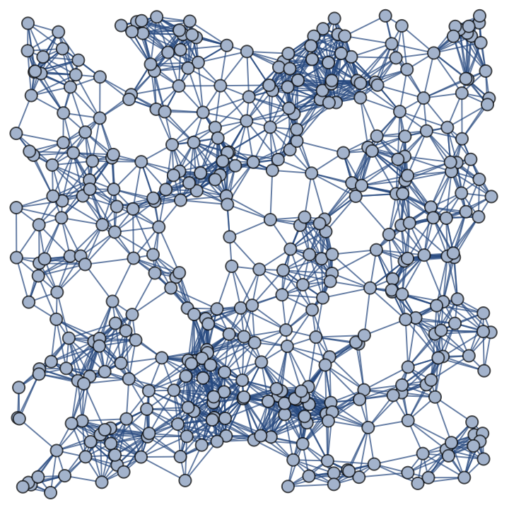
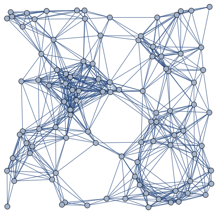
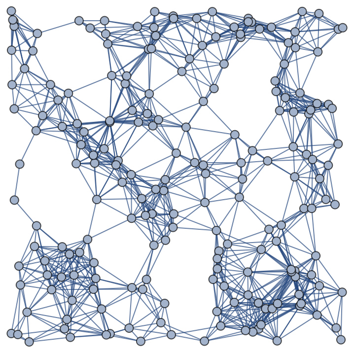
It can be noticed how, as the number of points grows, the discreteness scale decreases accordingly. This is necessary in order to avoid an excessive density of edges per vertex - an unnecessary computationally heavy task - as no extra information is contained in the edges as soon as the graph is completely connected. For illustration proposes, two sets of sprinklings with 100, 200, 300 and 400 vertices is provided, that differ only in the discreteness scale prefactor ). While all are embedded in the same underlying (flat) manifold, each sprinkling is different every time: this is done to ensure independence between every graph, so that every correlation to the coordinates is suppressed.
(b={1,1.2}
Out[]=
,
,
,
,
,
,
,
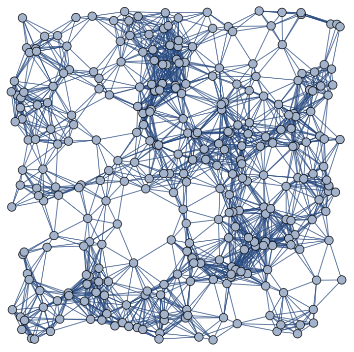
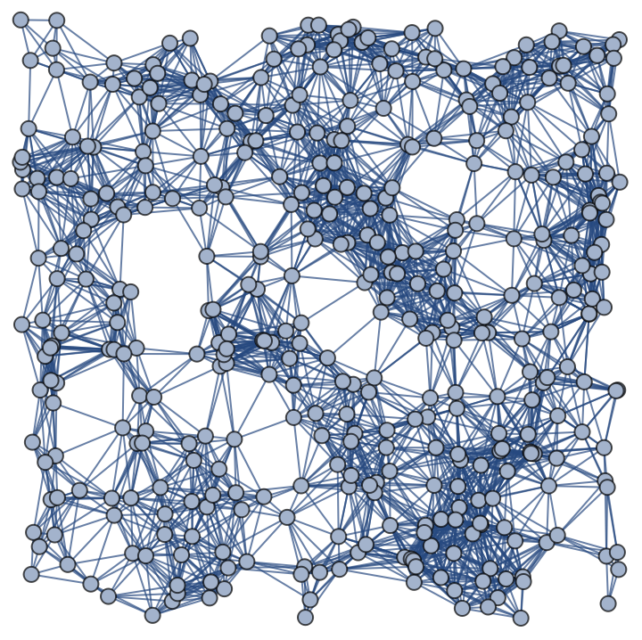
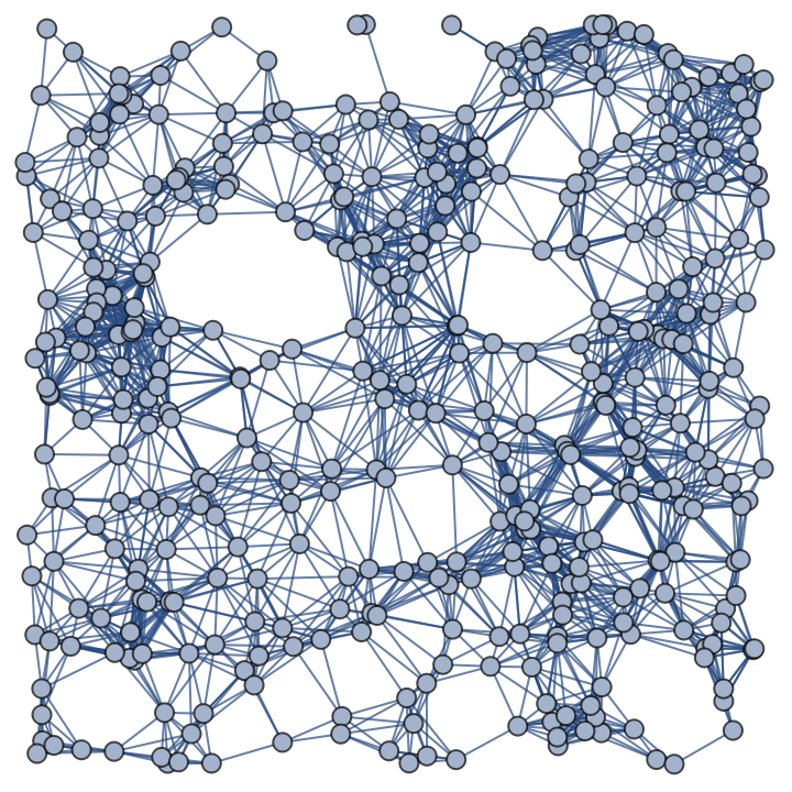
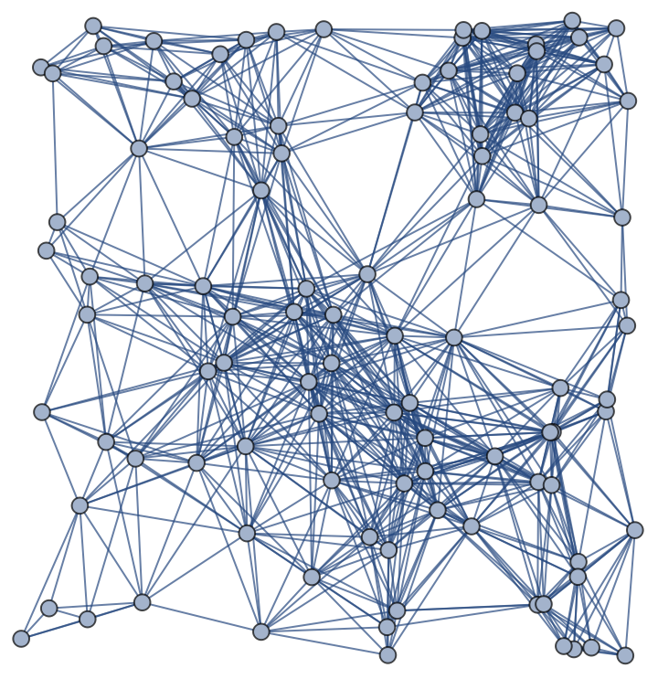
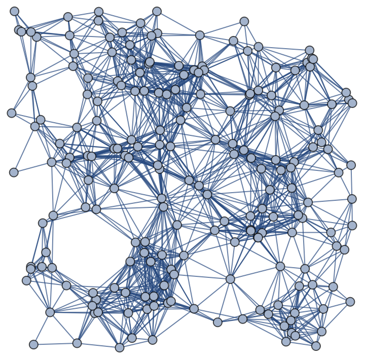
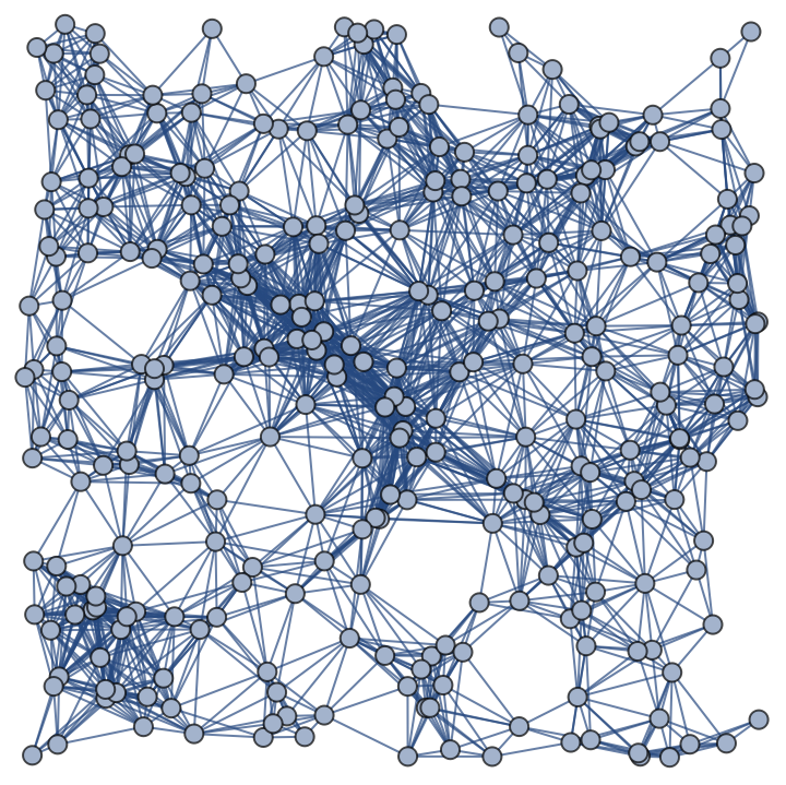
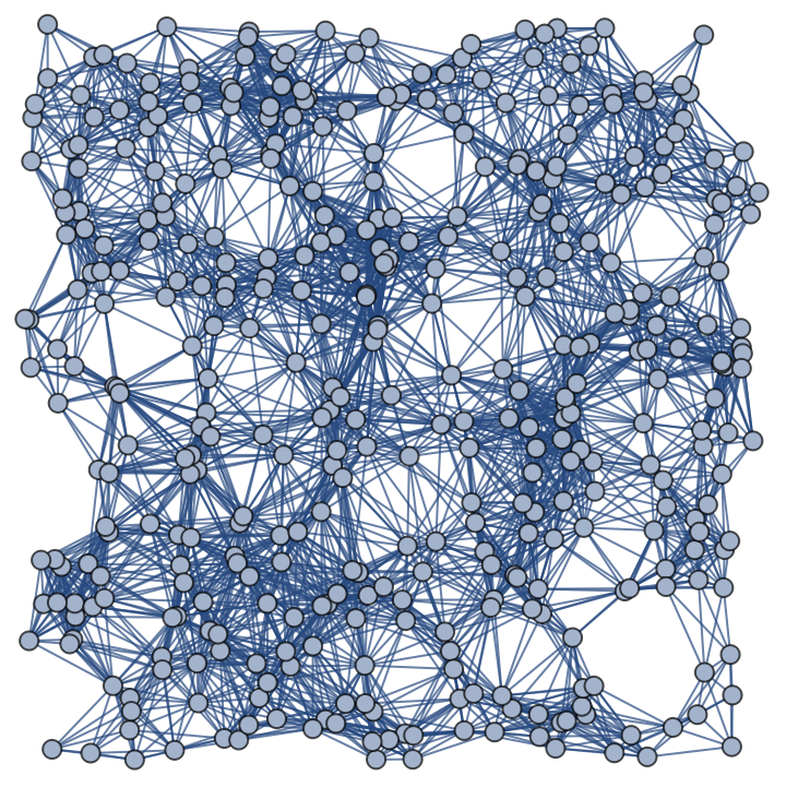
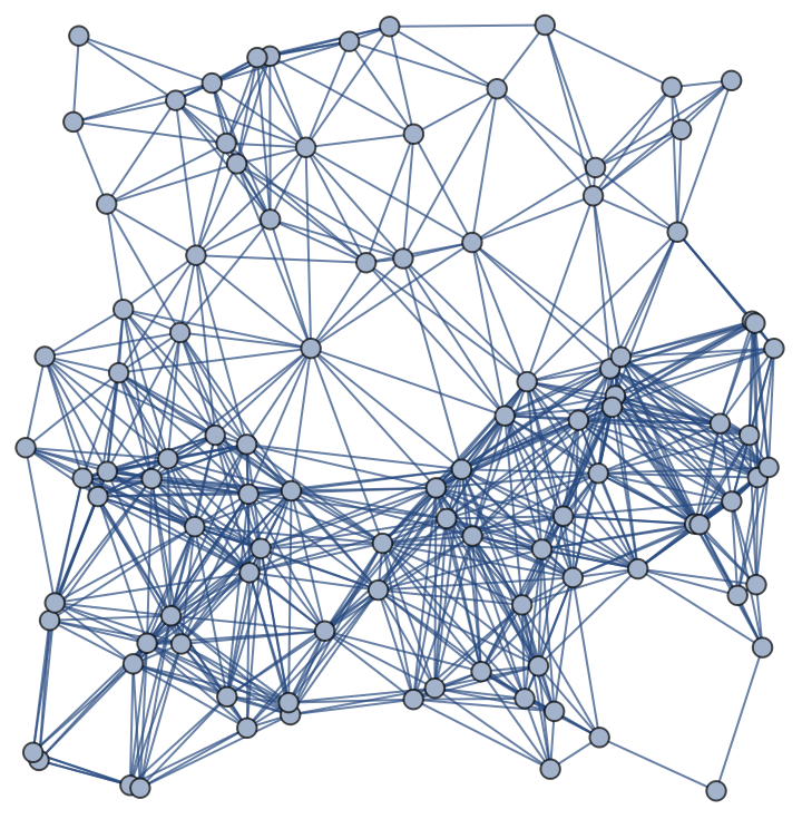
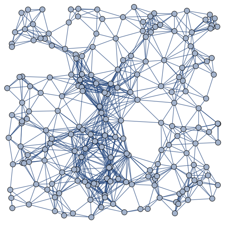
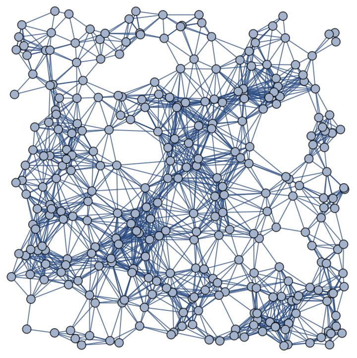
Of course, as the discreteness scale grows, so does the edge density. This is to be expected, as it basically means that the radius within which two vertices are to be considered connected grows as well. The same will happen for the scalarized version, that, as mentioned, will be implemented at the level of the norm. In particular, an extra parameter is added, which can be considered a coupling constant between the scalar field and the geometry (the norm) of the manifold. In pseudocode, two points will be connected by an edge if:
Norm[Between_two_Points]<discreteness_scale(1+coupling_constant**PDF[BinormalDistribution]).
-2
10
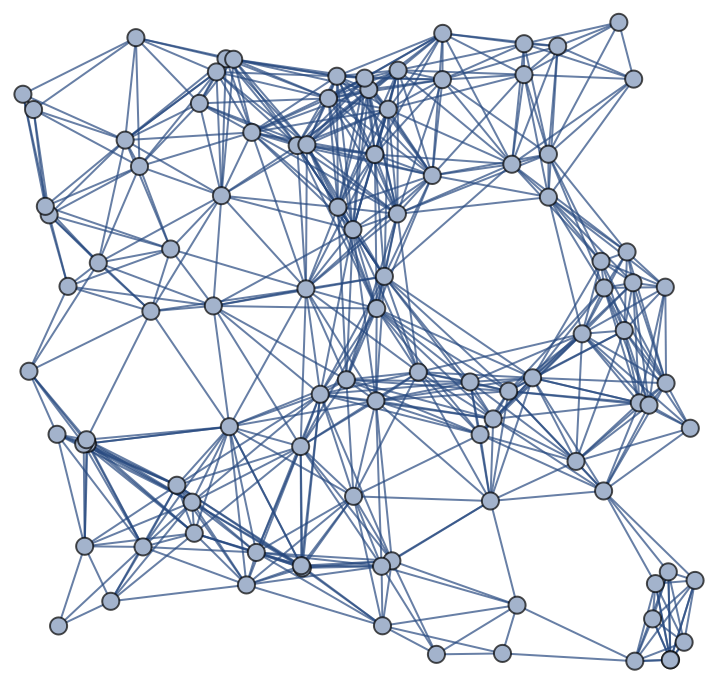
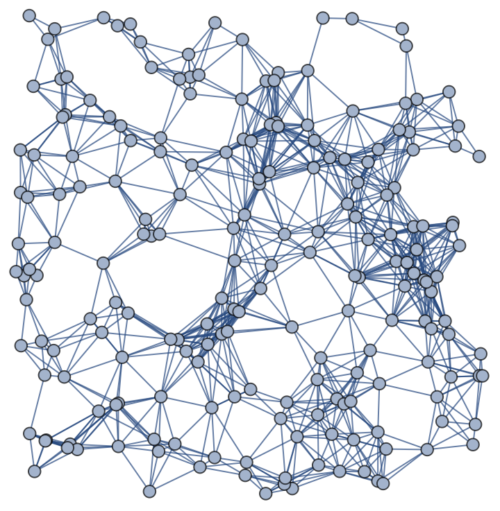
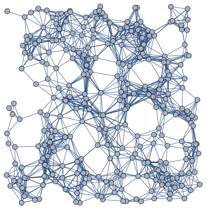
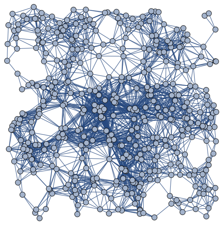
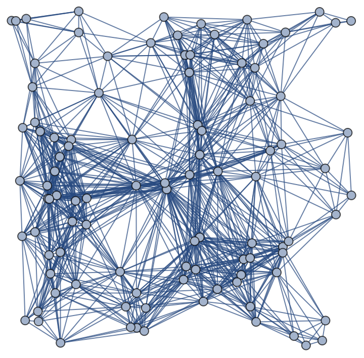
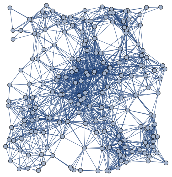
For illustration proposes, the result is visualised below: it is a set of two sets (one for each value of the discreteness scale) of (four, for increasing value of the sprinkling points count) spatial hypergraphs; each set is then recalculated for a new value of the coupling constant ). As before, every sprinkling is different, as it is generated every time independently from the ones before.
(c={0.08,0.12}
Out[]=
,
,
,
,
,
,
,
,
,
,
,
,
,
,
,
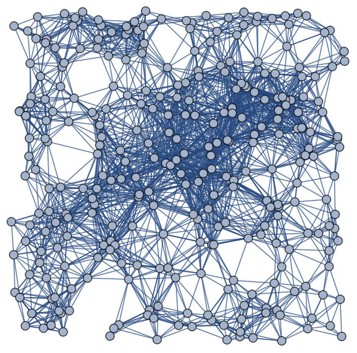
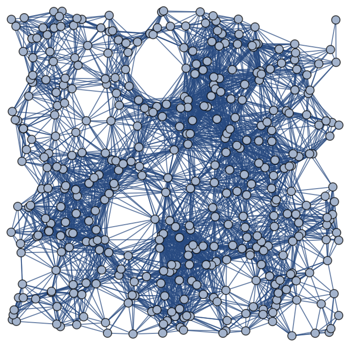
The effect of the scalar field is recovered by comparison of the vertex degree of each sprinkled point in the scalar configuration with the mean value of the respective non-scalarized one (with the same number of sprinkling points). As anticipated, this is allowed only in the case of flat spacetime, as the average of the vertex degree is only well-defined over the whole graph here.
The result is encouraging. The bell shape is clearly recovered, and – at least intuitively – the approximation appears to improve with both an increasing number of sprinkling points, and an increasing coupling constant. The second result in particular is to be expected, as the effects of the Scalar Field are obviously more prominent as it grows in value. The first one is reassuring: this approach seems to work fine, and one can therefore (at least) attempt to generalize it to curved spacetimes.
The (almost) monotonic behaviour of the plots confirm all the hopeful suspicions: increasing the number of sprinkled points yields a better approximation of the Scalar Field, as well as an increasing edge count and coupling constant. Again, the main focus has to be on the sprinkling: it is even possible (perhaps quite ambitiously) to claim that the asymptotics have an almost quadratic slope, a result that (a posteriori) justifies the assumption that the number of sprinkled points and the discreteness scale are in an inverse quadratic relationship with each other. The admittedly unexpected behaviour of the 400 sprinkling in the plot corresponding to an increased discreteness scale (for both values of the coupling constants) has to be investigated further: there is no reason to believe that the approximation would worsen with an increased number of sprinkled points, so the main hypothesis is that this is at best an artefact, and at worse a combined effect of the two other factors, that has to be better fine-tuned as they may possibly correlate. In trying to proceed with at least an additional point, a computational bottleneck was rapidly met, and therefore every additional consideration has to be postponed to a more fortunate (computationally speaking) circumstance.
Curved Manifold
Curved Manifold
The previous analysis was a moderate success, as it was also a necessary step to take before blindly trying to compute information in a spatial hypergraph that corresponds to a curved spacetime, where not only is the norm not uniform through the graph, but the curvature itself has relevant effects that need to be taken into account. Nevertheless, as for the Scalar Field, the actual shape of the intrinsic curvature has no reason to be a particularly significant factor. For the sake of generality, a curvature factor shall also be implemented in the algorithm, and the whole process (as was the case previously with the coupling factor) shall be run a second time for an increased intrinsic curvature (in the sense of absolute value).
The function defined to recover the sprinkling the curved manifold is, overall, the same as previously defined for the flat manifold, whereas additionally the curvature factor can be specified and the Repository function used to generate the vertices is “IntrinsicCurvedManifoldToGraph”. This essentially adds an extra layer to the resulting list, for the calculation is just repeated for a different value of the curvature factor. In the given example, the dimension of the list is [2,2,4], namely two (graphs for each value of the) curvature factor, two discretization scale prefactor and four sprinkled vertices count (same values as for the flat spacetime case).
There is nothing unusual to notice in this graphs; they are exactly as expected. Although unremarkable, it is worth mentioning the presences of unconnected vertices. This, while technically a problem when the vertices’ labels are dropped, is not particularly relevant in this case: as the focus is on the vertex degree, those unconnected vertices would only contribute zero to the total count; formally, the (lack of) meaning of an unconnected vertex in a spatial graph should be addressed, but as it is understood that it is only a problem of fine tuning of the discreetness scale, such subtleties are delayed to a later (perhaps more computationally capable) discussion. The same arguments apply as for the scalarized version, with the additional (and final) layer of the coupling constant (here again, the same values of the flat spacetime are used).
Neighborhood Vertices
Neighborhood Vertices
In the case of the flat spacetime sprinkling, it was quite straightforward to just compare the vertex degree of each sprinkled point in the scalar configuration with the mean value of the respective non-scalarized one. This is because the average of the vertex degree is only well-defined over the whole graph for a flat spacetime configuration. In the curved case, the norm is not uniform through the whole graph, and the fact that different sprinklings of the manifold are considered only worsens the situation. Once again, the fact that the coordinates labels are attached to each vertex will prove quite useful: as long as the sprinkled region is the same, there will always be a close enough neighborhood of a given point in which the norm would be uniform, and this neighborhood should not change for a different sprinkling of the same region. It is therefore reasonable to compare the vertices’ degree of each vertex only to the average of a neighborhood of vertices in that same region: in other word, for a given vertex in the scalarized configuration, its vertex degree is compared with the mean value of the vertices degree up to a certain number of edges away (in this project, it is assumed to be one, but it can be specified more generally) from the corresponding closest vertex in the non scalarized graph.
Conclusions
The results are, once again, encouraging, but much more evidently than the previous case, need to be expanded to acquire a certain level of significance. The subdivision of the following representation reflects the additional layer of the curvature factor, but is otherwise equivalent to the flat spacetime case.
This factually concludes this preliminary investigation. It has been verified that it is possible, within an increasing confidence range, to recover the effects of a Scalar Field directly from the vertex degree of a spatial hypergraph, at least when the vertices still conserve the vertices’ labels. A prospective on future applications and possible expansions of this project will conclude the analysis.
Future Applications
Future Applications
Asides from the already (multiple times) mentioned necessity of exploring this approach for an increasing number (and values) of the four parameters, another important prospective is the one to actually recover information about the presence of a Scalar Field without any previous assumptions on its presence, but only from hypothesis of the underlying metrics. In particular, it has been proposed to create a likelihood of such hypothesis, for instance considering some very well known and physically relevant metrics (Swartzchild, Kerr, Robinson-Walker, etc.). Both paths are only plausible with an increased level of computational capabilities, and as it has been already proposed to act on these possibility, an update of these results is already in production.
Complete Code
Functions
Functions
Program
Program
Acknowledgments
The author would like to thank Jonathan Gorard for his mentorship and moral support. They would also like to thank their group for the insightful conversations and the wonderful moments shared in together building these projects (and perhaps something more). In the person of Erin Cherry, they would finally thank the Wolfram Administration department for the very opportunity of being here.
References
◼
David Hilbert.'The Foundations of Physics (First Communication)'.In : Nachrichten von der Königlichen Gesellschaft der Wissenschaften zu Göttingen.Math.-phys.Klasse.(Nov.1915), Issue 8, p.395–407. Ed.by Jürgen Renn et al.Vol.250. The Genesis of General Relativity (Boston Studies in the Philosophy of Science).Dordrecht : Springer Netherlands, 2007. Chap.44, pp.1911–1924.
◼
Albert Einstein. ‘On the Relativity Principle and the Conclusions Drawn from it’. In: Jahrb. der Radioakt. und Elektron. 4 (Dec. 1907), p. 411-462. Trans. by Anna Beck. Vol. 2. The Collected Papers of Albert Einstein. Princeton University Press, 1989. Chap. 47, pp. 252–311
◼
Albert Einstein. ‘The Field Equations of Gravitation’. In: Königlich Preußische Akad. Wissenschaften, Sitzungsberichte (Nov. 1915). Trans. by Alfred Engel. Vol. 6. The Collected Papers of Albert Einstein. Princeton University Press, 1996, pp. 117–120
◼
Steven Weinberg. ‘The Principle of General Covariance’. In: Gravit. Cosmol. Princ. Appl. Gen. Theory Relativ. John Wiley and Sons, 1972. Chap. 4.1, pp. 91–93
◼
David Lovelock. ‘The Four-Dimensionality of Space and the Einstein Tensor’. In: Journal of Mathematical Physics 13.6 (June 1972), pp. 874–876.
◼
Charles W. Misner, Kip S. Thorne, and John Archibald Wheeler. ‘Stress-Energy Tensor and Conservation Laws’. In: Gravitation. 2nd ed. Princeton University Press, 2018. Chap. 5, pp. 130–163
◼
Israel Quiros et al. ‘The conformal transformation’s controversy: what are we missing?’ In: General Relativity and Gravitation 45.2 (Feb. 2013), pp. 489–518.
◼
T. Damour and G. Esposito-Farese. ‘Tensor-multi-scalar theories of gravitation’. In: Classical and Quantum Gravity 9.9 (Sept. 1992), pp. 2093–2176.
◼
1. Gorard, J. Some Relativistic and Gravitational Properties of the Wolfram Model. Complex Syst. 29, 599–654 (2020).